To start, I use Avogadro to build the geometry shown in Figure 5.32a and use it to construct the input file for an optimization with 4 constrained bond length. The values for the constraints are taken from a paper. Figure 5.32b shows the equilibrium geometry obtained with GAMESS, after 17 steps. Based on this geometry GAMESS finds the TS in three steps.
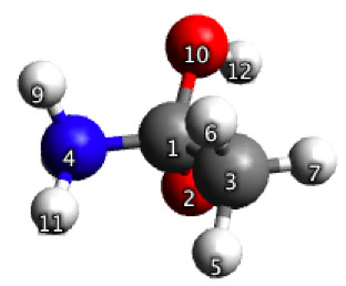
Figure 5.32a. Initial guess geometry for the constrained optimization discussed in Figure 5.33.
Click on the picture for an interactive version.
From Molecular Modeling Basics CRC Press, 2010
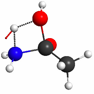
Figure 5.32b. The geometry resulting from the constrained optimization and the normal mode of the imaginary frequency computed for this structure at the PM3 level.
Click on the picture for an interactive version.
From Molecular Modeling Basics CRC Press, 2010
It will not always be possible to find an article that reports the TS structure for your reaction of interest. So let’s try to find the TS without the information from the article. I start from the same structure (Figure 5.32a), and I arbitrarily pick C1-O10 as the reaction coordinate constrained to 1.70 Å.
This constrained optimization results (after 23 steps) in the geometry shown in Figure 5.35a. The subsequent TS search results in the geometry shown in Figure 5.35b, which has no imaginary frequency and is clearly the product.

Figure 5.35a. The geometry resulting from a constrained optimization in which the distance between atoms 1 and 10 (see Figure 5.32a for numbering) was constrained to 1.7 Å, and the normal mode of the imaginary frequency computed for this structure at the PM3 level.
Click on the picture for an interactive version.
From Molecular Modeling Basics CRC Press, 2010
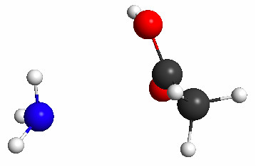
Figure 5.35b. The geometry resulting from a TS search initiated from the geometry shown in Figure 5.35(a).
Click on the picture for an interactive version.
From Molecular Modeling Basics CRC Press, 2010
The fact that the C–O bond is re-formed indicates that it should be stretched more in the initial guess, so I repeat the optimization with the C–O distance constrained to 2.0 Å instead of 1.70 Å. This results (after 39 steps) in the geometry shown in Figure 5.36. Using this as a starting geometry for the TS search leads to the TS in Figure 4.30a after 17 steps.

Figure 5.36. The geometry resulting from a constrained optimization in which the distance between atoms 1 and 10 (see Figure 5.32a for numbering) was constrained to 2.0 Å, and the normal mode of the imaginary frequency computed for this structure at the PM3 level.
Click on the picture for an interactive version.
From Molecular Modeling Basics CRC Press, 2010
In the screencast below I try to reproduce the calculations that lead to these figures. Because I rebuild the structure in Figure 5.32a, I get different starting coordinates, so the energies and number of steps are different than what I discuss in the book for the 4-constraints approach.
In the case of the 1-constraint approach, I actually manage to find the TS using the 1.70 Å constraint. Thus, the structures in Figures 5.35b and 5.36 do not appear in the screencast. This just goes to show how finicky TS searchers are to starting geometries.
While editing the screencast I noticed that the PM3 energies of the two TS structures I find are very different (11 kcal/mol). This is also true for the TSs I found when writing the book (where they are different by 6.6 kcal/mol).
This appears to be a problem that PM3 has with structures where bonds are partially broken or formed. I could not reproduce this for structures with normal bond lengths such as the reactants and products. Note that in the book, I use M06/6-31G(d) single point energies to compute barriers, and that the M06/6-31G(d)//PM3 single point energies of the TSs found with the two different method are only different by 0.03 kcal/mol.


7 comments:
An interesting variation on the TS you located is to add an extra water molecule, so that the proton transfer now occurs in a six-membered ring rather than four. Also of interest is to calculate the entropies for all the species to find out whether the entropy penalty resulting from the loss of a further six degrees of freedom for the extra molecule is compensated for by any enthalpic reduction. So, is the transition state with an extra water more or less likely than that with water merely as a remote spectator?
By the way, this is not merely an academic point. It is crucial for eg understanding how some enzymes work. For example Cytochrome P540.
Absolutely. In the book, I list water assisted proton transfer and alternative mechanisms (in this case, a step-wise mechanism) as the first things to check. Many proteases use a step wise mechanism with a tetrahedral intermediate.
Hi, do you know of any good solution for incorporating LaTeX labels into diagrams of molecular/atomic orbitals? I know of a few workarounds, such as manually overlaying LaTeX labels onto a pre-generated diagram, but I haven't found any solution that natively allows for that.
I don't use LaTeX, so I can't help you with that specific question.
I use screenshots (specifically SnapNDrag) to extract images from the programs, and then label the images in powerpoint. Then extract the labeled images again using screenshots.
To dhawk: Hi, you may be interested in the psfrag package form Latex. Psfrag substitutes your text marks with Latex objects (text, images). See a nice example here.
Your blog is invaluable. Do you have plans to post any tutorials for calculating the transition state of excited state reactions?
I am very happy to hear you find the blog useful!
I know very little about finding excited states and photochemistry.
What I do know is that transition state theory cannot be used to compute rate constants, because the molecule is not in thermal equilibrium with its surroundings. So, I don't really know what an excited state TS means, or if it has any meaning.
The bottom line is that I don't really know how to compute a rate constant (or, more accurately, the quantum yield) of a photochemical reaction, so I can't really blog about.
Post a Comment