Steric strain vs electrostatic attraction

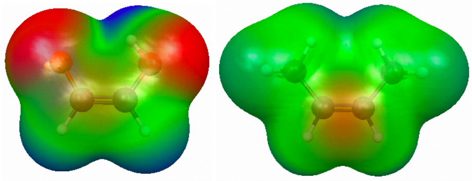
Figure 3.5. (a) RHF/6-31G(d) 0.002 au isodensity surface with superimposed electrostatic potential for (a) cis-HO(H)C=C(H)OH and (b) cis-CH3(H)C=C(H)CH3 and. In both cases, the maximum potential value is 0.05 au. (click on the picture for a bigger version).
From Molecular Modeling Basics CRC Press, May 2010.

This figure shows how the electrostatic potential superimposed on the 0.002 au isodensity surface can be used to rationalize why cis-HO(H)C=C(H)OH is more stable than trans-HO(H)C=C(H)OH, while the opposite is true for CH3(H)C=C(H)CH3.

The figure clearly shows the difference in polarity between hydroxyl and methyl groups. For the OH substitutent case the positive (O)H atom is close to the negative O(H) atom in the cis isomer. The CH3 group is non-polar and larger and the overlapping density indicates steric strain.

The figure is made with MacMolPlt as described in a previous post. Below is an interactive version made with Jmol (as described in a previous post). You'll notice that the color scheme is somewhat different, because Jmol maps the electrostatic potential value to a color in a different way than MacMolPlt. However, the general conclusion drawn from both programs is clearly the same.

Figure 3.5. (a) RHF/6-31G(d) 0.002 au isodensity surface with superimposed electrostatic potential for (a) cis-HO(H)C=C(H)OH and (b) cis-CH3(H)C=C(H)CH3 and.
Click on the picture for an interactive version

Electrostatic potential maps reloaded

Here is an interactive version of a figure I described in a previous post. Click on the picture to load it. Remember it's Jmol so you can rotate it and zoom as you like (Mac users: this works best with Safari).

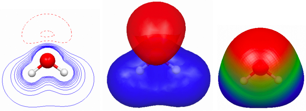
Figure 3.4. The RHF/6-31G(d) electrostatic potential of water.
Click on the picture for an interactive version

The Jmol animation loads a file (fig3-2-2.xyz), which you can access by right-clicking on the Jmol animation once you have loaded it (as described in a previous post). This file also contains all the necessary commands.

Figure 3.4.c is the most common depiction of electrostatic potential maps and the Jmol general syntax for the command for this is

isosurface 0.002 "density.cube.gz" color range -0.05 0.05 "potential.cube.gz"

The screencast below shows how I made the cube files that contain the electron density and electrostatic potential information using MacMolPlt. The first part is identical to the screencast in a previous post on obtaining the electron density cube file.

The program I used to convert the MacMolPlt file to a cube was written by Jonathan Gutow and can be download here.

I start by loading the RHF/6-31G(d) optimized geometry I computed for a previous post, and reorienting. The orientation makes it easier to define the plotting plane for the contour plots.

Electrostatic potential maps

Figure 3.4. (a) Contour plot of the electrostatic potential of H₂O. The maximum and minimum contour value is 0.5 Hartrees/electronic charge (au). (b) The corresponding 0.05 au isopotential surface. (c) The electrostatic potential displayed on the 0.002 au isodensity surface of water. The maximum (darkest blue) value corresponds to 0.05 au.
From Molecular Modeling Basics CRC Press, May 2010.

Here is a screencast of how I made the figure:

The files I used were created in a previous post. The various values specified above are determined using trial and error, i.e. I kept fiddling with it until it looked good to me. When using plots like this it is important to specify these values, because using different values can lead to very different looking plots.

Also, different programs use different color scales and color intensity to indicate positive and negative charge, so it is rarely possible to directly compare electrostatic potential maps from different programs.

See this post about using screen capture to get a file with the graphic. This was done for each plot, and the combined in a word processor.

The interactive version of this figure is the subject of a future post.

Electron density doesn't always tell the whole story

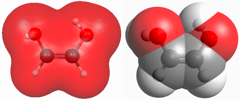
Figure 3.3. (a) RHF/6-31G(d) 0.002 au isodensity surface and (b) van der Waals surface of cis-HO(H)C=C(H)OH (click on the picture for a bigger version).
From Molecular Modeling Basics CRC Press, May 2010.

Looking at the electron density or the van der Waals surfaces one would expect steric strain in cis-HO(H)C=C(H)OH. (See this post on how to make such pictures and this post on how to make an interactive version such as the one shown below.)

However, contrary to CH₃(H)C=C(H)CH₃, the cis isomer is more stable than the trans isomer. This is of course due to the electrostatic attraction of the O and H atom in the hydrogen bond. Here the electron density tells only part of the story because this attraction involves the nuclei as well. Here an electrostatic potential map is more useful. How to make such plots will be the subject of future posts.

Figure 3.3. The RHF/6-31G(d) electron density of cis-HO(H)C=C(H)OH.
Click on the picture for an interactive version

Electron density and steric strain

Figure 3.2. (a) RHF/6-31G(d) 0.002 au isodensity surface and (b) van der Waals surface of cis-CH₃(H)C=C(H)CH₃ (click on the picture for a bigger version).
From Molecular Modeling Basics CRC Press, May 2010.

This figure shows how the electron density and van der Waals surfaces can be used to visualize steric strain. See this post on how to make such pictures and this post on how to make an interactive version such as the one shown below.

Figure 3.2. The RHF/6-31G(d) electron density of cis-CH₃(H)C=C(H)CH₃.
Click on the picture for an interactive version

Electron density reloaded

Here is an interactive version of a figure I described in a previous post. Click on the picture to load it. Remember it's Jmol so you can rotate it and zoom as you like (Mac users: this works best with Safari).

Figure 3.1. The RHF/6-31G(d) electron density of water.
Click on the picture for an interactive version

The Jmol animation loads this file (h2oprinc.xyz), which looks like this

3
jmolscript: script "http://propka.ki.ku.dk/~jhjensen/h2odensity.spt"
O -0.0000 0.0643 0.0000
H -0.7541 -0.5091 0.0000
H 0.7541 -0.5091 0.0000

and which, in turn, loads a script (h2odensity.spt), which looks like this

isosurface planex plane {0 0 0 0} contour 20 color absolute 0.002 0.05 "http://propka.ki.ku.dk/~jhjensen/h2oprinc.cube.gz"
delay 3
spin y 20
delay 10
spin off
isosurface planey plane {1 0 0 0} contour 20 color absolute 0.002 0.05 "http://propka.ki.ku.dk/~jhjensen/h2oprinc.cube.gz"
spin y 20
delay 10
spin off
isosurface planez plane {0 1 0 0} contour 20 color absolute 0.002 0.05 "http://propka.ki.ku.dk/~jhjensen/h2oprinc.cube.gz"
spin x 40
delay 10
spin off
isosurface threed 0.002 "http://propka.ki.ku.dk/~jhjensen/h2oprinc.cube.gz"
color isosurface red ; color isosurface translucent 0.15
spin y 20
delay 10
spin off
color isosurface red ; color isosurface translucent 0.5
select all; spacefill 100 %babel
spin y 20
delay 10
spin off

The screencast below shows how I made the cube file that contains the electron density information using MacMolPlt. The program I used to convert the MacMolPlt file to a cube was written by Jonathan Gutow and can be download here. In the screencast I mistakenly named the cube file h2odensity.cube.gz, but that's easy to change.

I start by loading the RHF/6-31G(d) optimized geometry I computed for a previous post, and reorienting. The orientation makes it easier to define the plotting plane for the contour plots.

Electron density

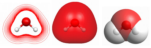
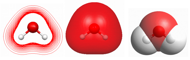
Figure 3.1. (a) A contour plot of the density of H₂O computed using RHF/6-31G(d). The maximum and minimum contour values are 0.05 and 0.002 aus. (b) The corresponding 0.002 au isodensity surface. (c) The surface corresponding defined by atomic spheres with van der Waals radii.
From Molecular Modeling Basics CRC Press, May 2010.

Here's a screencast about how I made the figure:

When making the contour plot (Figure 3.1.a) I pick 0.05 au as the maximum value (this will be the contour line closest to the nuclei) and 25 contour lines. This means that the spacing between the contour lines and thus the outer contour line will be 0.05/25 = 0.002 au.

Another, more common, representation of the density is a 3D version of one of the contour values: the isodensity surface (Figure 3.1.b). A common choice is 0.002 au, since that corresponds roughly to experimental estimates of molecular size, such as the van der Waals surface (Figure 3.1.c).

Unfortunately, MacMolPlt doesn't have a van der Waals display style, so I have to use Avogadro. This means I have to re-size (by eyeball) this part of the figure to make it the same size as the density plots. See this post about using screen capture to get a file with the graphic.

The interactive version of this figure is the subject of a future post.

A useful equation

(1)

This is a useful equation. Remember it, and your life will change for the better. The equation comes from one of the fundamental equations of statistical mechanics,

(2)

as you can see here

Both equations tell you how the energies of molecule A (E_A) and B (E_B) determine how many molecules of each (n_A and n_B) you will observe at equilibrium.

Eq (1) is simply a much more useful form of (2) for room temperature conditions, because it gives you a feel for what the relative energies mean in terms of chemistry. Yes, with a little practice you will be able to amaze and astound your friends.

An energy difference of 4.5 kcal/mol? Why, that means 0.001 times less B than A. 6.0 kcal/mol? 0.0001! The trick is to recognize that 1.36 is close enough to 1.5, and that 4.5/1.5 = 3 and 6.0/1.5 = 4, meaning that the energies correspond to concentration ratios of roughly 10^-3 and 10^-4, respectively. Respect, indeed! You'll be the life of the party.

You could of course use a calculator to get more accurate results, in which case you might as well use Eq (2). But if you routinely bring a scientific calculator to parties, then you have more serious problems to worry about anyway.

The astute reader will note that I made things pretty easy for myself by picking 4.5 and 6.0 kcal/mol, and that dividing, say, 5, by 1.5 is no mean feat. But at least you'll know that the answer is somewhere between 10^-3 and 10^-4, and that's often all you need.

If you believe in the metric system () you may prefer to work in kJ/mol, in which case 1.36 should be replaced by 5.70 and approximated by 6.

You can do the same party trick with rate constants by using transition state theory,

A barrier of 6 kcal/mol?, why that's a whopping 10⁹ per second! 20 kcal/mol? Here it's a good idea to sip your beer, to stall for time ... 0.1 s^-1, of course! I usually count by 3's (2 times 1.5), 2o is close to 21, 7 times 3, 14 times 1.5, meaning 10^13-14, 10^-1. Get me: I'm Richard Feynman!

On a different note, I firmly believe that animations similar to the screencast in this post could be used to make derivations much more accessible to students. I haven't been able to find any software to do this and I think this is a gaping hole in the world of software. I made the screen cast with Powerpoint, and there were many, many things I would change about if ppt would let me.

In case the notion of animated derivations strikes you as crazy, I leave you with a quote from Richard Feynman's aptly named book What Do You Care What Other People Think:

"When I see equations, I see the letters in colors – I don't know why. As I'm talking, I see vague pictures of Bessel functions from Jahnke and Emde's book, with light-tan j's, slightly violet-bluish n's, and dark brown x's flying around. And I wonder what the hell it must look like to the students."