Polarization and intermolecular interaction

Figure 4.16. 0.002 au isodensity surface with superimposed molecular electrostatic potential for (a) methane using the methane density for the methane–water dimer and (b) free methane monomer. The maximum potential value, 0.01 au, is five times smaller than in previous figures to make the increase in negative charge visible. The black spheres in (a) denote the position of the three nuclei of water. The level of theory is M06/6-31+G(2d,p)//M06/6-31G(d).
Click on the picture for an interactive version.
Click here for a pop-up window
From Molecular Modeling Basics CRC Press, 2010

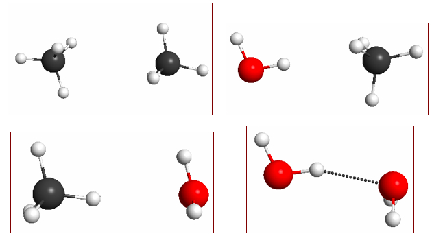
In a previous post I showed how the difference in the strengths of interaction between methane, methane-water, and water dimer is due to their differences in polarity, which can be visualized using molecular electrostatic potentials (MEPs). Methane interacts stronger with water than with methane because of polarization, i.e. rearrangement of the methane electrons due to the polar water molecule that, to a first approximation, induces a dipole moment in methane.

The polarization of the methane density is not visible in the MEP of the methane–water dimer (Figure 4.15b) because the polarity of the water H atom dominates the MEP in that region. But if we remove the water molecule, the net increase in negative charge in the methane molecule where it interacts with the partially positive H atom of the water is apparent (Figure 4.16).

Making the figure
This is a not a plot one makes every day, so the process is a bit involved. The main trick is to construct the methane part of the density from the corresponding localized molecular orbitals, and then tricking GAMESS into printing a file with just those LMOs that MacMolPlt can read. The procedure is described in some detail Section 5.5 of the book, so here I just post the corresponding screencast.

The book is out

The book is now available for purchase, at least in the States. You can order it directly from CRC Press or, for example, from Amazon.com (though not yet Amazon.co.uk). And why just one copy? Christmas is practically around the corner.

When molecules attract

Figure 4.14. M06/6-31G(d) optimized geometries of (a) methane dimer, (b) water–methane dimer where water acts as a H-bond donor, (c) water–methane dimer where methane acts as a H-bond donor, and (d) water dimer.
Click on the picture for an interactive version.
Click here for a pop-up window
From Molecular Modeling Basics CRC Press, 2010

The molecular dimers shown in Figure 4.14 have very different interaction energies: -0.5, -1.0, -0.6, and -5.1 kcal/mol, respectively; which are reasonably well reproduced at the M06/6-31+G(2d,p)// M06/6-31G(d) level of theory: -0.4, -0.5, 0.0, and -4.9 kcal/mol.

The source of this difference in intermolecular attraction can be easily visualized with electrostatic potential maps (Figure 4.15). Methane is non-polar and the main source of attraction in the methane dimer is dispersive forces (which are hard to visualize). Water is polar, and the methane–water interaction (where the water is the H-donor) is a bit stronger than the methane dimer. This is due to an electrostatic interaction - more specifically polarization, but more about this in a future post.

Figure 4.15. 0.002 au isodensity surface with superimposed molecular electrostatic potential for (a) methane dimer, (b) water–methane dimer where water acts as an H-bond donor, (c) water–methane dimer where methane acts as an H-bond donor, and (d) water dimer. The maximum potential value is 0.05 au and the level of theory is M06/6-31+G(2d,p)//M06/6-31G(d).
Click on the picture for an interactive version.
Click here for a pop-up window
From Molecular Modeling Basics CRC Press, 2010

Instructions on how to make interactive electrostatic potential maps with Jmol can be found here. Finally, I introduce a new feature (pop-up windows) to the blog because I can't figure out how to include Jmol buttons (which gives more control to the viewer) into blog posts. This feature also gives you access to the underlying GAMESS files as I have discussed here.

Double bonds - banana and otherwise

Figure 4.12. (a) B3LYP/6-31G(d) optimized geometry of ethene; (b) and (c) 0.045 au isosurfaces of the two localized banana MOs corresponding to the double bond.
Click on the picture for an interactive version
From Molecular Modeling Basics CRC Press, 2010

VSEPR theory can be used to explain structures of molecules with double and triple bonds, though this is rarely done in textbooks. Figure 4.12 shows some localized MOs for ethene, where the double bond is shown to consist of two curved MOs (sometimes called banana bonds), rather than the usual sigma and pi MOs. The banana LMOs are less spread out than single-bond LMOs, leading to less repulsion and an H–C–C angle larger than 109.5°, namely 116.3° [at the B3LYP/6-31G(d) level of theory].

Figure 4.13. 0.045 au isosurfaces of a localized pi MO [(a) top view and (b) side view] and two localized sigma bond MOs in benzene. The level of theory is B3LYP/6-31G(d).

Click on the picture for an interactive version
From Molecular Modeling Basics CRC Press, 2010

In the case of benzene the LMOs actually look like sigma and pi orbitals (Figure 4.13). Figure 4.13a and b are two views of the pi-bond LMO primarily between C4 and C5. Notice, however, that there is significant delocalization onto C3 and C6. There are identical pi-bond LMOs between C3 and C2 as well as C1 and C6, and the net result is an identical C–C bond length of 1.397 Å, roughly halfway between the CC bond length in ethane (1.531 Å) and ethene (1.331 Å).

I have discussed how to make these plots in a previous post.