Showing posts with label molecular workbench. Show all posts

Saturday, January 25, 2014

Protein unfolding at high temperature happens because of entropy


Here is a video in which I use Molecular Workbench to illustrate protein unfolding.  I then go on to explain how conformational entropy contributes to the spontaneous unfolding with increasing temperature. The videos are part of a series that I am working on.


This work is licensed under a Creative Commons Attribution 4.0 International License.

Saturday, January 18, 2014

Why is the heat capacity a maximum at a phase transition?


Here is a video in which I use Molecular Workbench to illustrate why the heat capacity is a maximum at a phase transition. The videos are part of a series that I am working on.


This work is licensed under a Creative Commons Attribution 4.0 International License.

Friday, December 13, 2013

Illustrating energy states and estimating enthalpy changes


Here are two videos in which I use Jmol and Molecular Workbench to illustrate energy states and MolCalc to estimate enthalpy changes. The videos are part of a series that I am working on.


This work is licensed under a Creative Commons Attribution 4.0 International License.

Friday, December 6, 2013

Thursday, September 6, 2012

Peer instruction questions for very basic molecular quantum mechanics

As I mentioned in my previous blog post I this year I made some screencasts of lectures to free up time for peer instruction questions.  Here are the peer instruction questions I used.


This time I tried Socrative for voting, which allows students to type in short answers to questions.  I can then select some of the questions and have students vote on their favorite.  This is what's happening in slide 13 and 23.

You'll notice I also made use of Molecule Calculator, which is introduced here.  Next year I have to remember also to assign the MolCalc intro video.


This work is licensed under a Creative Commons Attribution 3.0 Unported License.

Sunday, June 19, 2011

Peer instruction: mixing

These slides show questions I used when teaching mixing functions using peer instruction. The slides are in Danish, but I hope you get the idea and there is always Google translate. Any questions, just leave a comment.

Some comments about specific slides:
Slides 1-3 show results from a Molecular Workbench simulation, which you access here.  It is a variation on the simulation I used to illustrate entropy.  If you understand why the gas expands in that example, you also understand why the gasses mix.

Slides 4-10 show results from a Molecular Workbench simulation, which you access here.

Slides 4-5: after two votes there was no clear consensus, but most students likes A "no interactions between molecules".  The second vote came at the end of the first of three back-to-back lectures, so we had a third vote after the break.  There really was intense discussion of this during the break, when most finally settled on B "equal interactions between molecules".   I think A was popular because "ideal solution" conjures up an analogy to "ideal gas", but how can you have a liquid if there are no intermolecular attractions?

Slide 7-8: here is alternated between the simulation and the question a few times.  A better approach would have been to include the question on the web site with the simulation.

Related blog posts
See all posts related to peer instruction here.
Illustrating mixing
Simulations in teaching physical chemistry: thermodynamics and statistical mechanics

Thursday, May 19, 2011

Peer instruction: radial distribution functions

These slides show questions I used when teaching radial distribution functions using peer instruction. The slides are in Danish, but I hope you get the idea and there is always Google translate. Any questions, just leave a comment.

Some comments about specific slides:
Slide 8: The hint is given after the first vote.

Slides 11-18 show results from two Molecular Workbench exercises, which you can download here and here, once you have installed Molecular Workbench on your computer.

Slide 11: First I run the solid simulation, then pose the question and have a couple of votes, then click on the "show pair correlation function" in the MW simulation.  Note that you have to run for at least 100,000 fs to get good statistics (i.e. relatively smooth curves).  Then I explain the answer (slides 12 and 13)

Slide 14: Same procedure as slide 11, but for the liquid.

Slide 16: No vote, since the answer is pretty obvious, but I do ask where the peak at r = ~1.5 Å comes from.  Of course it comes from the attractive part of the Lennard-Jones potential, and you can clearly see some particles sticking together in the gas simulation.  To check, I change the depth of the well from 0.1 eV to 0.001 eV (simply double-click on any of the particles, and you will see what to do), re-run the simulation, and show the radial distribution function (summarized in slide 17).

See all posts related to peer instruction here.

Wednesday, May 18, 2011

Peer instruction: entropy

These slides show questions I used when teaching entropy using peer instruction. The slides are in Danish, but I hope you get the idea and there is always Google translate. Any questions, just leave a comment.

The slides refer to two Molecular Workbench simulations, which you can access here and here, and read more about here and here.

Specific comments to the slides
Slides 1-5: Here I start the simulation without removing the separator.  Then pose the question, two rounds of votes (usually not needed for the first simulation with 100 particles, as more than 80 % submit the correct answer), then remove the separator and explain.

Slides 10-15: Here I run the first simulation (small volume, low temperature) and carefully explain what the recorded times mean and how they correlate with probability.  Then I pose the first question (slide 10), two rounds of votes, then run the double volume simulation, then summarize the right answer (slide 11), and explain it (slide 12).  Same process for doubling the temperature.

See all posts related to peer instruction here.

Related blog posts
Illustrating entropy
Entropy, volume, and temperature
Simulations in teaching physical chemistry: thermodynamics and statistical mechanics

Saturday, December 4, 2010

Simulations in teaching physical chemistry: thermodynamics and statistical mechanics

In this post I summarize the simulations and I have used in teaching thermo and stat mech, and talk a bit about how I use them.

I co-teach two quite similar courses on this topic: one for nano-students and another for chemistry and biochemistry students.  In the nano course we use the book Molecular Driving Forces by Dill and Bromberg, and in the other Quanta, Matter, and Change by Atkins, de Paula, and Friedman.  At the end of this post I have organized the simulations by chapter for each book.

Some of simulations I have made (or modified extensively) and most of these have been discussed in previous blog posts, so I simply give the link to the respective blog post where there is more information.

The other simulations are from the Molecular Workbench (MW) library of models, and here I provide links that will open in MW, so you need to install MW before clicking on the links.  For some of them I also provide a brief description of what concepts try to demonstrate using the simulations.

How do I use the simulations?
All simulations are used during lecture to visualize concepts, start discussions, and motivate equations. I'll take Illustrating energy states as an example: instead of saying "Molecules in a gas translate, rotate, vibrate, and ....", I say "Here is a zoomed-in view of butane gas where you can see the molecules.  You can see that individual molecules move differently.  How do they move differently?  Anyone?  Right, they have different speeds.  This kind of motion is called translation.  What else? ..."

Practical tips
On a very practical note, my own simulations are all on web sites and I make sure to open all of them before the lecture, while I have all the MW simulations for the course indexed on a single MW page (click here to open in MW). It is not possible to embed these simulations in Powerpoint slides, but you can switch between Powerpoint and other applications without quitting Powerpoint (on a Mac you use command-tab and on Windows i believe it is windowskey-tab).  Note that you need access to the internet in the lecture room.

While I have screencasts of most of simulations on the blog posts, I don't use these during lecture.  I think it is too passive, and puts the students to sleep.  But I believe the screencasts are a good way for the students to review the main points of simulations after the lecture.  I put links to the blog posts on the course web site and in the lecture notes.

Is using simulations a good idea?
If possible I try to use a simulation within the first five minutes of a lecture, and have a maximum of 20 minutes between simulations.  I now only have one (45 minute) lecture left where I don't use a single simulation and I can just feel how I loose the student's attention after about 30 minutes.  You can just see it.  That being said, no one has ever mentioned the simulations in their course evaluations (good or bad), so I have no hard evidence that it improves my teaching.  But I can tell you that I enjoy lecturing much more with the simulations, so unless I get complaints I'll keep doing it. 

Making room for simulations in the lecture
I have taught the topics for many years without any simulations, and was never at a loss for material to cover.  Lecture time is precious, and these simulations take time to present and discuss.  You really have to introduce the simulation carefully (don't rush this part!) before you start them, and very often you want the students to speculate about what will happen before you start them.  Furthermore, they tend to stimulate many more questions, that you can hopefully turn into a discussion instead of simply answering them, than derivations - that's the whole point.

So how do you "make room" for the simulations?  I have cut out most of the derivations from the lectures.  To pay for my sins, I provide relatively detailed (typed) lecture notes ahead of lecture (I generally don't use Powerpoint), which include step-by-step derivations. So I'll say things like "Starting with these assumptions we can write down this equation.  This can be rewritten as this equation, which is much simpler.  The details on how we got from here to there are in your notes, but note that in step 3 we assume that ... which is an approximation."  No complaints so far.  If only more progress had been made on simulating derivations ...

Here are the simulations organized by chapter

Molecular Driving Forces by Dill and Bromberg (1st edition)

Ch 6: Entropy and the Boltzmann distribution law
Illustrating entropy

Ch 10: Boltzmann distribution law
Polymer unfolding: The book uses two simple bead models of polymers in this chapter to illustrate micro and macrostates and model protein melting.  I use this example extensively both in lectures and homework problems.  So I made this simulation to illustrate how higher energy macrostates become more likely at higher temperatures.


Ch 11: Statistical mechanics of simple gasses and solids
Illustrating energy states
Energy states in the water molecule: a slightly more complicated molecule than HCl (used in Illustrating energy states) with more than one vibrational mode and 3 rotational degrees of freedom.
Internal energy and molecular motion
Entropy, volume, and temperature


Ch 12: Temperature, heat capacity
The molecular basis of differential scanning calorimetry: heat capacity and energy fluctuations

Ch 13: Chemical equilibria
Seeing chemical equilibrium (opens in MW)
Dalton's law of partial pressure (opens in MW)


Ch 14: Equilibria between solids, liquids, and gasses
Seeing specific and latent heat (opens in MW): I use this simulation to illustrate how the same substance can be solid, liquid, and gas depending on the temperature.
A gas under a piston (opens in MW): I use this simulation to show that, for example, decreasing the pressure can have the same effect as increasing the temperature.
The phase diagram explorer (opens in MW)
Raoult's law: ideal solutions (opens in MW): Here, I use the simulation of the pure liquid to illustrate vapor pressure.


Ch 15: Solution and Mixtures
Mixing gasses, and mixing of ideal and non-ideal liquids
Raoult's law: ideal solutions (opens in MW)
Raoult's law: negative deviation (opens in MW) 
Raoult's law: positive deviation (opens in MW)


Ch 16: Solvation and transfers of molecules between phases
Visualizing osmotic pressure in an osmotic equilibrium (opens in MW)
Desalination using reverse osmosis (opens in MW)


Quanta, Matter, and Change by Atkins, de Paula and Friedman (1st edition)

Ch 13: The Boltzmann distribution
Illustrating energy states
Energy states in the water molecule: a slightly more complicated molecule than HCl (used in Illustrating energy states) with more than one vibrational mode and 3 rotational degrees of freedom.
Internal energy and molecular motion

Ch 14: The first law of thermodynamics#
The molecular basis of differential scanning calorimetry: heat capacity and energy fluctuations
  
Ch 15: The second law of thermodynamics
Illustrating entropy
Entropy, volume, and temperature
  
Ch 16: Physical equilibria
Seeing specific and latent heat (opens in MW): I use this simulation to illustrate how the same substance can be solid, liquid, and gas depending on the temperature.

A gas under a piston (opens in MW): I use this simulation to show that, for example, decreasing the pressure can have the same effect as increasing the temperature.

The phase diagram explorer (opens in MW)
Raoult's law: ideal solutions (opens in MW): Here, I use the simulation of the pure liquid to illustrate vapor pressure.
Visualizing osmotic pressure in an osmotic equilibrium (opens in MW)
Desalination using reverse osmosis (opens in MW)

Ch 17: Chemical equilibria#
Seeing chemical equilibrium (opens in MW)
Dalton's law of partial pressure (opens in MW)

# I don't teach this part of the course, but if I did I would use these simulations

Related posts:
An Atkins Diet of Molecular Workbench 
One, Two, Three, MD 
Tunneling and STM (a first stab at using Molecular Workbench to teach quantum mechanics)

Illustrating mixing

This screencast shows Molecular Workbench simulations I have made to illustrate mixing.

The first simulation illustrates the mixing of 2 ideal gases, which mix readily.  Since the gas particles don't interact you can think of the mixing as each gas expanding to fill both containers independently of each other.  As I have shown in this simulation, the driving force for this expansion is an increase in entropy.  Therefore, the driving force for mixing two ideal gasses is also purely entropic.
The second set of simulations illustrates the mixing of 2 liquids.  Since they are liquids there must be attractive interactions between the atoms.  If there were no interactions they would be (ideal) gasses.  The strength of the interactions (and the temperature) determine whether they mix or not.

In the first liquid simulation, the attraction between two green atoms (εGG), between two blue atoms (εBB), and between a green and a blue atom (εGB) are the same.
This means that a green atom doesn't care whether it is sitting next to a blue atom or another green atom.  The net effect is that green and red atoms are equally likely to be on the right or left side of the container, and the liquids mix for the same reason as the ideal gasses mix: the driving force is purely entropic. That means the enthalpy of mixing is zero:
This is the definition of an ideal mixture (or ideal solution).  The two liquids will mix at any temperature.

In the second liquid simulation, the attraction between two blue atoms (εBB) is stronger than between two green atoms (εGG) and between a green and a blue atom (εGB).
Note that the ε's are negative: a smaller ε means a stronger attraction.  This means that the blue particles would rather be with other blue particles, i.e. the enthalpy increases if the particles are mixed.
(z is the number of contacts between particles in solution, and xG is the mole fraction of green atoms).  This is an example of a non-ideal mixture, where the definition for a non-ideal mixture is
Because ΔmixH > 0 this non-ideal solution mixes spontaneously (i.e. ΔmixG < 0) only for
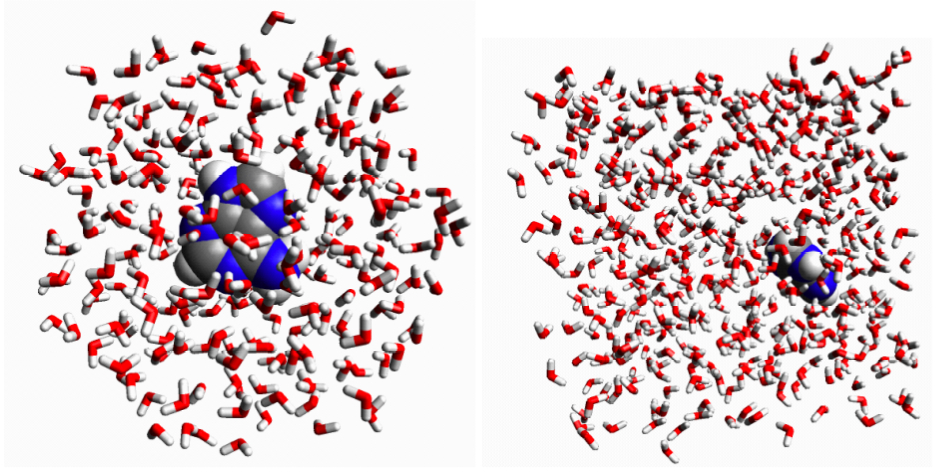
Oil and water is a common example of such an non-ideal mixture: the oil-oil interactions are stronger than the oil-water and water-water interactions.

Salt and water is another example of on idea mixture, but here ΔmixH <  0 so salt and water almost always mixes spontaneously.  The interpretation is that the interactions between the salt ions and water is stronger than the average interaction between salt ions and between water molecules.
Implications and limitations
The definition of ΔmixH in terms of the ε's suggest that liquids should also mix if
which would be a more general definition of an ideal mixture.

This is tested in the third liquid simulation.  As you can see the liquids mix more than in the second simulation, but not quite as much as in the first simulation.  This is mostly because of the simulation runs only for 100 picoseconds, which is to short to mix fully.  But another reason is that there is less space (on average) between the blue atoms compared to the green atoms, because the blue atoms attract each other more.  The next effect is that the blue particles tend to stay together to lower the enthalpy.  More mathematically,  z (the number of contacts between particles in solution) is not exactly the same for the blue and green particles so the interpretation of ΔmixH in terms of the ε's breaks down.  The "safest" definition of an ideal mixture thus remains:
i.e. "like dissolves like".

Accessing the simulations
You can play around with the simulations here and here, or you can download the models here and here if you have Molecular Workbench installed on your computer.

Saturday, November 6, 2010

The molecular basis of differential scanning calorimetry: heat capacity and energy fluctuations


Melting and boiling points are convenient and important measures of stability.  But how do you measure a melting point of, for example, nanoparticles that are too small to see?

This screencast shows two Molecular Workbench simulations (you can find them here and here) I made [see credits at the end of the post] to illustrate the connection between phase transitions, changes in heat capacity, and energy fluctuations, and the slides below takes you through the basic ideas behind them.

Slide 1: In the first simulation heat is added to a nano-particle and the resulting temperature increase is measured. When viewing the simulation notice that the temperature increases less during the melting/evaporation.

Slide 2: To analyze the data we first switch the x and y-axes, so that heat added (i.e. the internal energy, U) is plotted as a function of temperature.

Slide 3: The data is a bit noisy (mainly because the simulation heats the particle too fast: from 0 to almost 3000 K in about 200 picoseconds!), so I smooth it by fitting a curve to it.

Slide 4: From the smoothed data I can calculate how fast the energy changes with temperature.  This is the heat capacity (Cv), which peaks at a temperature around 1350 K - the melting temperature of the particle.

Slide 5: This observation forms the basis of differential scanning calorimetry, which measures the temperature as a function of the flow of energy to a system, and determines the melting point by finding the temperature where the heat capacity peaks.

Slide 6: One way to explain why the heat capacity peaks at a phase transition such as melting is through its relation to energy fluctuations: the system changes most during a phase transition ("bonds" between particles are broken and formed), so the energy fluctuates more, meaning that the heat capacity is largest.

Slides 7, 8, and 9: In the second set of simulations the energy is plotted a function of time at 3 temperatures: before the particle melts (500 K), when the particle melts/evaporates (1350 K), and after the particle has evaporated (3000 K).

Slide 10: Results from the 3 simulations are compared.  Clearly the fluctuations are largest when the temperature is 1350 K.  The fluctuations at 3000 K are larger than at 500 K, even though the heat capacities are similar.  This is because the heat capacity is proportional to the average energy fluctuation divided by the temperature squared (slide 6).
You may wonder why we don't see two heat capacity peaks: one for melting and one for evaporation.  This is because of the particle is so small (i.e. composed of relative few particles).  For a macroscopic systems (like water) the phase transitions are well defined.  Water is ice at 272 K, melts at 273 K, and is a liquid at 274 K (at 1 atmosphere of pressure); and the heat capacity has a very narrow peak at 273 K. As particles become smaller their phase transitions become less well defined, the heat capacity peak becomes broad, and in some cases (like this one) you get a single heat capacity peak for melting and evaporation.  This means that the phase transition cannot really be classified as melting or evaporation and that is occurs over a relatively large temperature range.  Li and Truhlar have an interesting article on this subject. If you would like to play around with or modify the simulations they can be downloaded here and here, but you need to download Molecular Workbench first. Credits: The simulations are based on models and scripts by Arie Aziman and Carlos Gardena, who based their work on a model by Dan Damelin, i.e. they are made possible, like Molecular Workbench itself, by open source science.

Saturday, October 2, 2010

Illustrating energy states


Here is a screencast showing 2 simulations I made to illustrate energy states (often also called microstates).  Open any book on statistical mechanics and you'll see a formula like this (for the Boltzmann distribution),
and, perhaps, a figure much like this.
But what are these "energy states" and ε's exactly? Hopefully the screencast and associated simulations, which you can find here and here, will help make this clearer.

About the simulations
If you want to play around with the HCl simulation, note that you have to reload the page if you want to change the translational motion.  This simulation is made with Jmol.  The molecular dynamics simulation of butane is made with Molecular Workbench.

Sunday, August 29, 2010

Entropy, volume and temperature


This screencast shows a Molecular Workbench simulation I made to illustrate the connection between entropy, volume, and temperature.


Each simulation runs for 50 picoseconds (ps) and records how much time the two particles spend together (as a dimer) and apart (as monomers).  These times are a reflection of the relative probabilities of the dimer (pdimer) and monomers (pmonomers).
In the first simulation of the screencast the particles spend 38.3 ps together and 11.7 ps apart.  When I double the volume (while keeping the temperature constant) in the second simulation, the particles spend 32.7 ps together and 17.3 ps apart.


This makes intuitive sense: when the particles are not together they have a harder time finding each other again in a bigger volume.  Put another way, the probability is lower that the particles find each other when they move in a larger volume.


Now I want to connect this intuitive explanation with a thermodynamic one (i.e. an explanation in terms of free energy and entropy) :


The relative probability of being together and apart is given by the change in free energy (ΔA) on going from the dimer to the two monomers (dimer -> 2 monomers)
The increase in pmonomers/pdimer (from 0.31 to 0.53) on doubling the volume must mean that ΔA  decreases when the volume is doubled.  Statistical mechanics tells us that the only thermodynamic term in A that is affected by volume (V) is the translational entropy
 and that an increase in volume will increase the entropy of a particle
So when the volume is doubled the entropy of each particle (the dimer and each monomer) is increased by Rln(2). As a result ΔS for the reaction dimer -> 2 monomers increases [by Rln(2)] and ΔA = ΔU - TΔS decreases by RTln(2).  So the probability of the dimer relative to the monomers decrease because the entropy is increased when the volume increases.


In the last simulation of the screencast I double the temperature (while keeping the volume constant) compared to the first simulation. As a result the particles now spend less time together (19.2 ps) than apart (30.8 ps).

This also makes intuitive sense: the dimer is more likely to be struck by a particle with a kinetic energy larger than the potential energy that is holding it together: Furthermore, when the monomers happen to collide they are more likely to have a combined kinetic that is larger than the potential energy holding the dimer together, i.e. "with too much kinetic energy to stick together".

As before, this must mean that ΔA decreases when the temperature is increased.  The increase in translational entropy due to temperature is indeed larger than for the volume
and consistent with the observed larger change in the time the particles spend apart.

If you think of the dimer as a crude model of a salt you want to dissolve, this explains why dilution (increasing the volume) or heating increases the solubility (the amount you can dissolve).  Conversely, increasing the concentration (the amount of particles per volume) or decreasing the temperature helps dimer formation and, in a larger sense, self assembly.

You can play around with it on this web page, or you can download the model if you have Molecular Workbench installed on your computer. Enjoy!

Clarifications and approximations
 You may wonder why I discuss the Helmholtz free energy change (ΔA; some books use ΔF) rather than the Gibbs free energy change, when the volume changes.  This is because the volume of the system (i.e. the two compartments) does not change. Another argument is that no work is done during the expansion.

I have implicitly invoked the ergodic hypothesis which states that the probability computed using a collection of molecules at a single instant in time is equal to the probability computed for a single molecule over a long period of time.  While it makes intuitive sense, I don't believe this has been rigorously proven.

Related blog posts
Illustrating entropy
Where does the ln come from in S = k ln(W)?

Sunday, March 14, 2010

Illustrating Entropy


This screencast shows some Molecular Workbench models I made to illustrate entropy.

In the first model a monatomic gas consisting of 100 particles are initially restricted to the left container, but when the separator is removed the gas expands to fill both containers evenly, on average.

The temperature is held constant during the simulation, so the internal energy (which equal to the temperature times a constant) stays constant. The driving force behind the expansion is therefore purely entropic.

Using two simpler cases with two and three particles, I show that the probability of having NL particles (out of N total) on the left is

where W is the weight or the number of equivalent combinations of particles in two containers. The screencast goes on to show that W is largest when the gas is evenly distributed between the two containers, so that is what happens when the separator is removed because that is the most probable thing to happen.

For N particles and two containers the number of combinations if there are NL particles in the left container is

(as explained here and here).

As in the simpler cases, the most likely state for 100 particles is an equal distribution of particles among the two containers (NL = 50). The main difference between 3 and 100 particles is that in the former case you'll occasionally (2/8 or 25 % of the time) see all particles in one container, whereas for 100 particles you'll never (2 x 10-28 % of the time) see all particles in one container.

Entropy, S, is defined as

where kB is Boltzmann's constant. This function is largest when W is largest, so one can say that the gas expands to maximize its entropy, but it's a bit like saying the gas expands because that is the most probable.

The change in entropy is

which can be approximated using the more usual equation for the entropy change upon doubling the volume of an ideal gas while keeping the temperature constant

(The latter equation becomes more accurate as the number of particles increase, because it relies on Stirling's approximation).

The model is too wide to fit in this blog but you can play around with it on this web page, or you can download the model if you have Molecular Workbench installed on your computer. Enjoy!

Related blog posts
Where does the ln come from in S = k ln(W)?
Entropy, volume, and temperature

Wednesday, March 3, 2010

Internal energy and molecular motion


This screencast shows a Molecular Workbench model I made to illustrate the connection between internal energy and molecular motion (the model is included at the bottom of the post).

For a monatomic gas such as He or Ar the part of the internal energy (U) that depends on temperature (T) is
and has only contributions from translational motion. Kinetic theory tells us that
which, with a little algebra, gives us a direct connection between the internal energy and the average kinetic energy of the atoms in the gas:
You can see in the first container that while the internal energy reflects an average speed, the individual atoms can have very different speeds, which are constantly changing due to collisions. This can be illustrated by coloring the atoms according to the kinetic energies (red means more kinetic energy).

Increasing the temperature increases the internal energy and this is reflected in an increase in the average speed, as you can see by clicking on the "Increase T" button.

However, it is important to remember that the internal energy is a reflection of the kinetic energy, which is also a reflection of the mass. Thus, a heavier atoms will have the same internal energy and kinetic energy at the same temperature, but the atoms will move slower on average (the "Increase M" button).

Also, the internal energy can be increase by adding more particles, but this does not change the average speed of the molecules at the same temperature (the "Increase n" button).

The last ("Diatomic") button changes the atoms to diatomic molecules without changing the mass, i.e. the mass of the atoms in the second container are half that of the atoms in the first container. Because the mass is unchanged the average speed of the molecules (more precisely, of their center of mass) is the same as for the atomic gas at the same temperature, as is the translational internal energy (3/2nRT ).

However, notice that the molecules are also rotating, meaning they have additional (internal) energy compared to the atomic gas, which amounts to nRT (3/2nRT for non linear molecules):
The internal energy also has a vibrational contribution (here the frequency is converted to a wavenumber, i.e. units of cm-1):
though it is hard to make out the vibrational motion in the simulation. However, for most diatomic molecules this contribution is negligible at temperatures relevant to most chemists.

You can play around with the model yourself by clicking on the picture below, or on this web page, or you can download the model if you have Molecular Workbench installed on your computer. Enjoy!


Tuesday, February 16, 2010

One, two, three, MD

Some exciting developments over at the Molecular Workbench (MW) blog run by MW author Charles Xie. I have several blog posts on MW, but it was necessary to install MW to check it out for yourself. Now it is possible to embed a MW applet in web pages (and blog posts!) like the one here (just push the play button!):
I think this is a big step forward for MW. While it is easy to download and install MW, it still removed MW a few clicks from the user and made it "appear to be yet another kind of annoying pop-up" and Charles notes. It's very easy to do this. The screencast below shows how I made the simulation above in MW. Note that it literally takes one minute (and 5 seconds). When you hit save you get two files: md.cml and md$0.mml. I transferred these to my web server where I had also put the MW applet (mwapplet.jar). The html code is <applet code="org.concord.modeler.MwApplet" archive="mwapplet.jar" height="300" width="100%"><param name="script" value="page:0:import md.cml"></applet> To include it in a blog, where mwapplet.jar is not installed, add the server address in front of mwapplet.jar and md.cml, e.g. http://myserver.edu/md.cml.

Wednesday, January 27, 2010

It's all about boundaries

Fig3-8
Figure 3.8. (a) Adenine (C5H5N5) in a liquid drop of 246 water molecules. (b) Adenine in a periodic box of 511 water molecules.
From Molecular Modeling Basics CRC Press, May 2010.

Conceptually, the simplest way of simulating a molecule in solution is to place it in the middle of a roughly spherical ball of water molecules (Figure 3.8a) and perform an molecular dynamics simulation.

One problem is this approach is that the drop would eventually evaporate if the simulation is run long enough. Another problem with the liquid drop model is that the water molecules at the surface of the drop do not behave like water molecules in liquid water.

Therefore, most explicit solvation simulations use periodic boundary conditions (Figure 3.9).

Fig3-9
Figure 3.9. Sketch of periodic boundary in two dimensions: (a) The position of the particles in the central box are copied and placed in neighboring boxes. Figure 3.8b shows a cube from a real simulation. (b) When a molecule tries to leave the box during an MD simulation, it reappears at the opposite end of the box, so the number of particles in the central box stays constant.
From Molecular Modeling Basics CRC Press, May 2010.

You can find interactive versions of Figures 3.8a and 3.9b here (I am grateful to Kestutis Aidas for providing the coordinates).

Click on the picture for an interactive version

And you can find an animated version of Figure 3.9 here (an example of where a movie really is worth 10,000 words).


The animation was made with Molecular Workbench (MW). You can play with the simulation here or you can download the MW file here (after you gave installed MW).

Saturday, September 26, 2009

Tunneling and STM


A few weeks ago, I gave a guest lecture (read: "I am at a conference that day, could you do it for me?") in a course entitled Unifying Concepts in Nanoscience. The topic was basic quantum mechanics (chapter 9 and a bit of 10 in Atkin's Physical Chemistry): particle in a box, etc.

These days, the first thing I do when preparing a lecture is to scour Molecular Workbench for useful animations, as I have discussed in a previous post. True to form MW did not disappoint, and I put together the following set of MW slides (note: you need to install MW first before clicking on it).

The screencast above shows how I used four of the slides to illustrate the concept of tunneling and and how it applies to STM.

Once again, I found animated simulations in general, and MW in particular, invaluable in bringing across complex concepts. And once again MW did all the hard work.

2012.09.01 UpdateI made a few more screencasts of parts of my lecture

Saturday, June 6, 2009

An Atkins diet of Molecular Workbench


In a recent post I showed an example of how to use Molecular Workbench (MW) in a p-chem lecture. The idea with that post was to keep it simple. Here I'll tell you what I actually prepared for the lectures, but the main point is really to draw your attention to the MW simulations, which are simply wonderful.

I had two back-to-back 45 minute lectures to cover chapter 16 in Atkins et al.'s Quanta, Matter, and Change on physical equilibria, i.e. phase changes and diagrams, chemical potential, colligative properties, ideal solutions, activity, etc.

So, I scoured MW for simulations related to these topics and created a new MW document with a list of the simulations I wanted to show during lecture (the screencast shows how), which can be found here. If you use MW as your "browser" loading new simulations is much faster than, say, powerpoint.

I'll say it again: rhe main point of this post is really to draw your attention to the MW simulations, which are simply wonderful. They really bring rather abstract points (like the deviation from non-ideality) or complex behavior (like osmosis) to life, and helps keep everyone awake (including myself). I should say that thermodynamics was not why I fell in love with science.

Btw, we're using Atkins Quanta for the first time, and I find it a great improvement over his P-Chem book in the thermo-department. Most references to steam engines and phase rules are relegated to various addenda in the back of the chapters. This was clearly a painful decision, as this quote attests to

"One [point] is that one of the most celebrated results in chemical thermodynamics. the phase rule, can be used as a basis of discussing the implications of the phase diagram, but it is not essential. It is described in Further Information 16.1."

I always found lecturing on steam engines and other celebrated results of thermodynamics a bit like Mr. Burn's attempt to send a telegram to the Prussian Embassy in Siam by first aerogyro: a tad dated. And on that note, I believe it is time to 23-skidoo.