The Polarity and Solvation option in MolCalc

+Maher Channir, under the capable supervision of MolCalc designer +Jimmy Charnley Kromann, has added a great new feature to the Molecule Calculator, shown in the video below.



Some technical stuff
The solvation energy, molecular surface area, and dipole are computed using the PM3/PCM interface recently implemented in GAMESS by +Casper Steinmann.  The displayed surface, which is slightly different than that used by GAMESS, is computed by JSmol, which also computes the eletrostatic potential based on charges computed by OpenBabel when making a mol2 file.

Amide hydrolysis, revisited

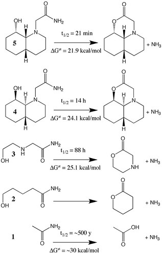
Figure 4.29. Sketch of hydrolysis reaction of several amides together with their experimentally observed half-lives. The free energies of activation are computed via Equations (4.30) and (4.31). (Adapted from N. M. Hernandes et al 2008. Journal of Organic Chemistry 73: 6413–6416.)
From Molecular Modeling Basics CRC Press, 2010
January, 2011 update: The figure in the book is missing an N atom in structures 4 and 5

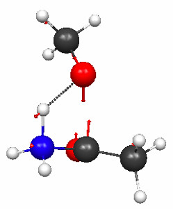
Figure 4.30a and b shows the TS geometries for the hydrolysis of 1 and 3 computed at the PM3 level of theory, together with the normal modes associated with the imaginary frequencies (2336i and 239i cm^–1, respectively).

Figure 4.30a. PM3 geometries of the TSs for hydrolysis of compound 1 (Figure 4.29), and the normal modes associated with the imaginary frequencies.

Click on the picture for an interactive version.

From Molecular Modeling Basics CRC Press, 2010

Figure 4.30b. PM3 geometries of the TSs for hydrolysis of compound 3 (Figure 4.29), and the normal modes associated with the imaginary frequencies.

Click on the picture for an interactive version.

From Molecular Modeling Basics CRC Press, 2010

As I show in the book, the predicted activation free energy of 1 is 4.2 kcal/mol higher than the activation free energy for the hydrolysis of 3. The source of the difference is roughly half electronic (1.9 kcal/mol) and half thermodynamic (2.3 kcal/mol). The explanation for the latter is the loss of translational entropy associated with hydrolysis of 1, but it is not obvious why the electronic activation energy should be lower.

For example, one might imagine that it would be energetically unfavorable to fold the chain of 3 into a ring due to some kind of strain when forming the transition state. This can be tested by studying the hydrolysis of 2 (Figure 4.29), which should have roughly the same amount of ring-strain associated with the reaction.

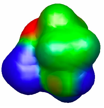
Indeed, the free energy of activation for hydrolysis of 2 is considerably higher than that for 3, and due entirely to an increased electronic activation energy.  This points toward the importance of the amine group in the middle of the chain in lowering the electronic barrier for 3-hydrolysis, presumably by stabilizing the partially positive –NH₃⁺-like portion of the TS (Figure 4.31).

Figure 4.31. 0.002 au isodensity surface with superimposed molecular electrostatic potential of the TS for hydrolysis of 3. The maximum potential value is 0.05 au, and the level of theory is M06/6-31G(d). The orientation is the same as Figure 4.30.

Click on the picture for an interactive version.

From Molecular Modeling Basics CRC Press, 2010

It might be tempting to ascribe the more open TS structure in 3 compared to 1 (Figure 4.30) to ring-strain, but the TS for “methanolysis” of 1 is equally open (Figure 4.32). This is presumably due to steric hindrance of the methanol methyl group and the carbonyl oxygen.

Figure 4.32. PM3 geometries of the TSs for methanolysis of compound 1 (Figure 4.29), and the normal modes associated with the imaginary frequencies.

Click on the picture for an interactive version.

From Molecular Modeling Basics CRC Press, 2010

I will discuss how to find the TS structure for the hydrolysis of 1 in a future post.  I have already discussed how to find the TS structure for the hydrolysis of 3 here and here.  This post describes how to verify that the TS connects the correct reactants and product, and this post describes the relationship between half lives and activation free energy.

Polarization and intermolecular interaction

Figure 4.16. 0.002 au isodensity surface with superimposed molecular electrostatic potential for (a) methane using the methane density for the methane–water dimer and (b) free methane monomer. The maximum potential value, 0.01 au, is five times smaller than in previous figures to make the increase in negative charge visible. The black spheres in (a) denote the position of the three nuclei of water. The level of theory is M06/6-31+G(2d,p)//M06/6-31G(d).
Click on the picture for an interactive version.
Click here for a pop-up window
From Molecular Modeling Basics CRC Press, 2010

In a previous post I showed how the difference in the strengths of interaction between methane, methane-water, and water dimer is due to their differences in polarity, which can be visualized using molecular electrostatic potentials (MEPs). Methane interacts stronger with water than with methane because of polarization, i.e. rearrangement of the methane electrons due to the polar water molecule that, to a first approximation, induces a dipole moment in methane.

The polarization of the methane density is not visible in the MEP of the methane–water dimer (Figure 4.15b) because the polarity of the water H atom dominates the MEP in that region. But if we remove the water molecule, the net increase in negative charge in the methane molecule where it interacts with the partially positive H atom of the water is apparent (Figure 4.16).

Making the figure
This is a not a plot one makes every day, so the process is a bit involved. The main trick is to construct the methane part of the density from the corresponding localized molecular orbitals, and then tricking GAMESS into printing a file with just those LMOs that MacMolPlt can read. The procedure is described in some detail Section 5.5 of the book, so here I just post the corresponding screencast.

When molecules attract

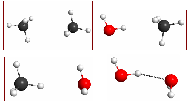
Figure 4.14. M06/6-31G(d) optimized geometries of (a) methane dimer, (b) water–methane dimer where water acts as a H-bond donor, (c) water–methane dimer where methane acts as a H-bond donor, and (d) water dimer.
Click on the picture for an interactive version.
Click here for a pop-up window
From Molecular Modeling Basics CRC Press, 2010

The molecular dimers shown in Figure 4.14 have very different interaction energies: -0.5, -1.0, -0.6, and -5.1 kcal/mol, respectively; which are reasonably well reproduced at the M06/6-31+G(2d,p)// M06/6-31G(d) level of theory: -0.4, -0.5, 0.0, and -4.9 kcal/mol.

The source of this difference in intermolecular attraction can be easily visualized with electrostatic potential maps (Figure 4.15). Methane is non-polar and the main source of attraction in the methane dimer is dispersive forces (which are hard to visualize). Water is polar, and the methane–water interaction (where the water is the H-donor) is a bit stronger than the methane dimer. This is due to an electrostatic interaction - more specifically polarization, but more about this in a future post.

Figure 4.15. 0.002 au isodensity surface with superimposed molecular electrostatic potential for (a) methane dimer, (b) water–methane dimer where water acts as an H-bond donor, (c) water–methane dimer where methane acts as an H-bond donor, and (d) water dimer. The maximum potential value is 0.05 au and the level of theory is M06/6-31+G(2d,p)//M06/6-31G(d).
Click on the picture for an interactive version.
Click here for a pop-up window
From Molecular Modeling Basics CRC Press, 2010

Instructions on how to make interactive electrostatic potential maps with Jmol can be found here. Finally, I introduce a new feature (pop-up windows) to the blog because I can't figure out how to include Jmol buttons (which gives more control to the viewer) into blog posts. This feature also gives you access to the underlying GAMESS files as I have discussed here.

I'm positive

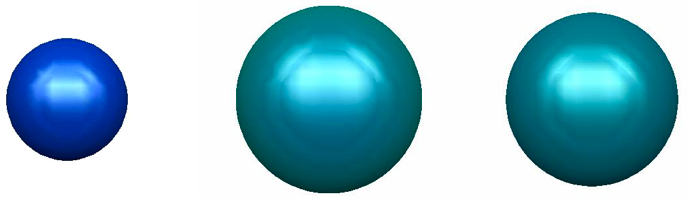
Figure 4.2. 0.002 au isodensity surface with superimposed electrostatic potential of (a) Li⁺, (b) Na⁺, and (c) K⁺ ion. The maximum potential value is 0.8 au, and the level of theory is B3LYP/6-31G(d).
From Molecular Modeling Basics CRC Press, May 2010.

Here is an example of how computational chemistry can be used to enhance teaching at the general chemistry level.

Why does the ionization energy decrease on from Li to Na to K? That's the same as asking why the electron affinities decrease on going from Li⁺ to Na⁺ to K⁺.

Figure 4.2 show the ions colored by how positive they are at the surface (i.e. the electrostatic potential superimposed on the 0.002 isodensity surface). The darker the
color the more positive the ion, and it is clear that the Li+ ion is “more positive” than Na⁺, which is more positive than K⁺. Thus, more energy should be released when adding an electron to Li⁺ compared to Na⁺, and hence more energy is needed to remove an electron from Li
compared to Na (and similarly for K).

The reason why Li⁺ is “more positive” than Na⁺ or, more accurately, why the potential on the 0.002 au isodensity surface is more positive for Li⁺ than for Na⁺, is that the former is a smaller ion than the latter, so the surface is closer to the +1 charge at the center of the ion.

Figure 4.4. 0.002 au isodensity surface with superimposed electrostatic potential of (a) Li⁺, (b) Ne⁺, and (c) Na⁺ ion. The maximum potential value is 0.8 au, and the level of theory is B3LYP/6-31G(d).
From Molecular Modeling Basics CRC Press, May 2010.

This rationalization is, of course, only qualitative and is is not predictive of the ionization energies among different groups. For example, based on Figure 4.4 one would expect that Ne would have roughly the same ionization potential as Na, which is not true at all.

When making these figures it is very important to get the relative sizes of the ions correct, but this can be difficult since each image can be zoomed to an arbitrary size. The screencast below shows how to control this in MacMolPlt using the Manual Windows Parameter window.

The same point can also be made with a "quick-and-dirty" electrostatic potential, as shown in this interactive figure. Here the electrostatic potential is due to a plus one charge centered at the atom (rather than the nuclear charge and the electron density) and the surfaces are the spheres defined by empirical ionic radii. The Jmol script can be found here, and the mol2 files here, here, and here.

Click on the picture for an interactive version

I have my moments

Figure 3.7. Contour plot of the RHF/6-31G(d) electrostatic potential and 0.002 au isodensity surface of (a) CH₃COO^-, (b) HF, and (c) F₂. The maximum/minimum contour values are, respectively, 0.5/0.025; 0.1/0.005; and 0.005/0.00025 au respectively. Blue corresponds to a negative potential. In each case the outer-most contour looks like the corresponding contour in the electrostatic potential due to a charge, dipole, and quadrupole, respectively.
From Molecular Modeling Basics CRC Press, May 2010.

This figure makes 3 points:

1. It shows what the electrostatic potential of a charge, dipole, and quadrupole looks like.

2. It show the relative strengths of the electrostatic potentials due to a charge, dipole, and quadrupole.

3. It shows that the electrostatic potential of a charge, dipole, and quadrupole deviates significantly from the actual electrostatic potential near the molecular surface.

Here is a screencast showing how I made Figure 3.7a. (If I were to do it over I would have chosen red for negative and blue for positive... oh, well.)

Here is an interactive version of the figure. Click on the picture to load it. Remember it's Jmol so you can rotate it and zoom as you like (Mac users: this works best with Safari).

Figure 3.7. The RHF/6-31G(d) electrostatic potentials of acetate, HF and F₂.
Click on the picture for an interactive version

See these two posts (here and here) on how to make plots like that with Jmol. From a Jmol perspective the only new thing is that I show two isosurfaces simulateneously. This is done by loading the file twice to create two "frames" that Jmol can display simultaneously. You can find the script file with all the commands here, but the general syntax is:

load files file1.xyz file2.xyz
frame 1.1; isosurface surf1 plane {0 0 0 0} contour 40 color range -0.05 0.05 "potential.cube.gz"
frame 2.1; isosurface surf2 0.002 "density.cube.gz" 

Even though you want a 2D contour plot of the potential, it is necessary to make a 3D cube file. Because I use unusually low cutoffs to show the outer contours, I had to trick MacMolPlt into making a bigger grid. I show how on the screencast below.

Quick and dirty electrostatic potential maps

In a previous post I showed how to compute an electrostatic potential map superimposed on the 0.002 isodensity surface of a molecule based on data computed using quantum chemical methods such as RHF/6-31G(d).

Previous posts (such as this one) have demonstrated that the van der Waals surface is a reasonable substitute for the 0.002 isodensity surface. Similarly, the electrostatic potential due to atomic charges can be a reasonable substitute for the electrostatic potential due to the electronic density.

The screencast above shows how to make such electrostatic potential maps using Avogadro and Jmol.

Avogadro uses an empirical method to determine the atomic charges (an integral part of the MMFF force field). It is possible to change the surface using the so-called "Iso Value" but I could not find any documentation on how that actually works. An Iso Value of 0 seems to correspond to the van der Waals sphere surface. It is currently not possible to alter the color range as far as I can see.

Jmol is not able to determine the charges, but the information can be transferred from Avogadro by saving a mol2 file. The electrostatic potential option in the Jmol menu corresponds to the following set of commands (as far as I can determine):

isosurface solvent color range -0.05 0.05 map mep
color isosurface translucent 0.5

and this set of commands can thus be used to control the color range and the nature of the surface. The default surface is a solvent accessible surface, which is slightly larger than the van der Waals surface.

A static and interactive version of the Avogadro and Jmol electrostatic potential map, respectively, can be found here.

Electrostatic potential map made with Avogadro
Click on the picture for an interactive version made with Jmol

Related blogpost: The polarity and solvation option in MolCalc

Steric strain vs electrostatic attraction

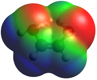
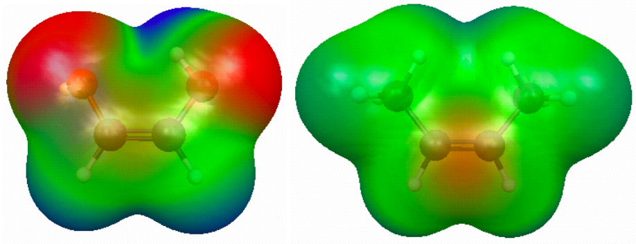
Figure 3.5. (a) RHF/6-31G(d) 0.002 au isodensity surface with superimposed electrostatic potential for (a) cis-HO(H)C=C(H)OH and (b) cis-CH3(H)C=C(H)CH3 and. In both cases, the maximum potential value is 0.05 au. (click on the picture for a bigger version).
From Molecular Modeling Basics CRC Press, May 2010.

This figure shows how the electrostatic potential superimposed on the 0.002 au isodensity surface can be used to rationalize why cis-HO(H)C=C(H)OH is more stable than trans-HO(H)C=C(H)OH, while the opposite is true for CH3(H)C=C(H)CH3.

The figure clearly shows the difference in polarity between hydroxyl and methyl groups. For the OH substitutent case the positive (O)H atom is close to the negative O(H) atom in the cis isomer. The CH3 group is non-polar and larger and the overlapping density indicates steric strain.

The figure is made with MacMolPlt as described in a previous post. Below is an interactive version made with Jmol (as described in a previous post). You'll notice that the color scheme is somewhat different, because Jmol maps the electrostatic potential value to a color in a different way than MacMolPlt. However, the general conclusion drawn from both programs is clearly the same.

Figure 3.5. (a) RHF/6-31G(d) 0.002 au isodensity surface with superimposed electrostatic potential for (a) cis-HO(H)C=C(H)OH and (b) cis-CH3(H)C=C(H)CH3 and.
Click on the picture for an interactive version

Electrostatic potential maps reloaded

Here is an interactive version of a figure I described in a previous post. Click on the picture to load it. Remember it's Jmol so you can rotate it and zoom as you like (Mac users: this works best with Safari).

Figure 3.4. The RHF/6-31G(d) electrostatic potential of water.
Click on the picture for an interactive version

The Jmol animation loads a file (fig3-2-2.xyz), which you can access by right-clicking on the Jmol animation once you have loaded it (as described in a previous post). This file also contains all the necessary commands.

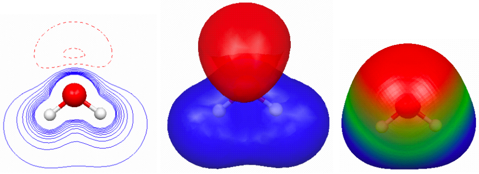
Figure 3.4.c is the most common depiction of electrostatic potential maps and the Jmol general syntax for the command for this is

isosurface 0.002 "density.cube.gz" color range -0.05 0.05 "potential.cube.gz"

The screencast below shows how I made the cube files that contain the electron density and electrostatic potential information using MacMolPlt. The first part is identical to the screencast in a previous post on obtaining the electron density cube file.

The program I used to convert the MacMolPlt file to a cube was written by Jonathan Gutow and can be download here.

I start by loading the RHF/6-31G(d) optimized geometry I computed for a previous post, and reorienting. The orientation makes it easier to define the plotting plane for the contour plots.

Electrostatic potential maps

Figure 3.4. (a) Contour plot of the electrostatic potential of H₂O. The maximum and minimum contour value is 0.5 Hartrees/electronic charge (au). (b) The corresponding 0.05 au isopotential surface. (c) The electrostatic potential displayed on the 0.002 au isodensity surface of water. The maximum (darkest blue) value corresponds to 0.05 au.
From Molecular Modeling Basics CRC Press, May 2010.

Here is a screencast of how I made the figure:

The files I used were created in a previous post. The various values specified above are determined using trial and error, i.e. I kept fiddling with it until it looked good to me. When using plots like this it is important to specify these values, because using different values can lead to very different looking plots.

Also, different programs use different color scales and color intensity to indicate positive and negative charge, so it is rarely possible to directly compare electrostatic potential maps from different programs.

See this post about using screen capture to get a file with the graphic. This was done for each plot, and the combined in a word processor.

The interactive version of this figure is the subject of a future post.