Wednesday, December 30, 2009

Quick and dirty electrostatic potential maps


In a previous post I showed how to compute an electrostatic potential map superimposed on the 0.002 isodensity surface of a molecule based on data computed using quantum chemical methods such as RHF/6-31G(d).

Previous posts (such as this one) have demonstrated that the van der Waals surface is a reasonable substitute for the 0.002 isodensity surface. Similarly, the electrostatic potential due to atomic charges can be a reasonable substitute for the electrostatic potential due to the electronic density.

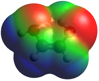
The screencast above shows how to make such electrostatic potential maps using Avogadro and Jmol.

Avogadro uses an empirical method to determine the atomic charges (an integral part of the MMFF force field). It is possible to change the surface using the so-called "Iso Value" but I could not find any documentation on how that actually works. An Iso Value of 0 seems to correspond to the van der Waals sphere surface. It is currently not possible to alter the color range as far as I can see.

Jmol is not able to determine the charges, but the information can be transferred from Avogadro by saving a mol2 file. The electrostatic potential option in the Jmol menu corresponds to the following set of commands (as far as I can determine):
isosurface solvent color range -0.05 0.05 map mep
color isosurface translucent 0.5
and this set of commands can thus be used to control the color range and the nature of the surface. The default surface is a solvent accessible surface, which is slightly larger than the van der Waals surface.

A static and interactive version of the Avogadro and Jmol electrostatic potential map, respectively, can be found here.

Electrostatic potential map made with Avogadro
Click on the picture for an interactive version made with Jmol

Related blogpost: The polarity and solvation option in MolCalc

Tuesday, December 29, 2009

Steric strain vs electrostatic attraction

Fig3-2-3
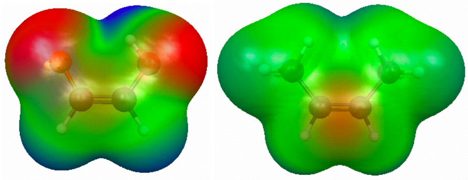
Figure 3.5. (a) RHF/6-31G(d) 0.002 au isodensity surface with superimposed electrostatic potential for (a) cis-HO(H)C=C(H)OH and (b) cis-CH3(H)C=C(H)CH3 and. In both cases, the maximum potential value is 0.05 au. (click on the picture for a bigger version).
From Molecular Modeling Basics CRC Press, May 2010.

This figure shows how the electrostatic potential superimposed on the 0.002 au isodensity surface can be used to rationalize why cis-HO(H)C=C(H)OH is more stable than trans-HO(H)C=C(H)OH, while the opposite is true for CH3(H)C=C(H)CH3.

The figure clearly shows the difference in polarity between hydroxyl and methyl groups. For the OH substitutent case the positive (O)H atom is close to the negative O(H) atom in the cis isomer. The CH3 group is non-polar and larger and the overlapping density indicates steric strain.

The figure is made with MacMolPlt as described in a previous post. Below is an interactive version made with Jmol (as described in a previous post). You'll notice that the color scheme is somewhat different, because Jmol maps the electrostatic potential value to a color in a different way than MacMolPlt. However, the general conclusion drawn from both programs is clearly the same.

Figure 3.5. (a) RHF/6-31G(d) 0.002 au isodensity surface with superimposed electrostatic potential for (a) cis-HO(H)C=C(H)OH and (b) cis-CH3(H)C=C(H)CH3 and.
Click on the picture for an interactive version

Sunday, December 27, 2009

Electrostatic potential maps reloaded

Here is an interactive version of a figure I described in a previous post. Click on the picture to load it. Remember it's Jmol so you can rotate it and zoom as you like (Mac users: this works best with Safari).
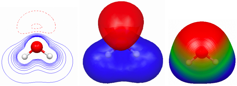
Figure 3.4. The RHF/6-31G(d) electrostatic potential of water.
Click on the picture for an interactive version

The Jmol animation loads a file (fig3-2-2.xyz), which you can access by right-clicking on the Jmol animation once you have loaded it (as described in a previous post). This file also contains all the necessary commands.

Figure 3.4.c is the most common depiction of electrostatic potential maps and the Jmol general syntax for the command for this is
isosurface 0.002 "density.cube.gz" color range -0.05 0.05 "potential.cube.gz"
The screencast below shows how I made the cube files that contain the electron density and electrostatic potential information using MacMolPlt. The first part is identical to the screencast in a previous post on obtaining the electron density cube file.

The program I used to convert the MacMolPlt file to a cube was written by Jonathan Gutow and can be download here.

I start by loading the RHF/6-31G(d) optimized geometry I computed for a previous post, and reorienting. The orientation makes it easier to define the plotting plane for the contour plots.

Saturday, December 26, 2009

Wishlist

Christmas is only 363 days away. It's never to early to start working on a new wish list.


Monday, December 21, 2009

Electrostatic potential maps

Fig3-2-2
Figure 3.4. (a) Contour plot of the electrostatic potential of H2O. The maximum and minimum contour value is 0.5 Hartrees/electronic charge (au). (b) The corresponding 0.05 au isopotential surface. (c) The electrostatic potential displayed on the 0.002 au isodensity surface of water. The maximum (darkest blue) value corresponds to 0.05 au.
From Molecular Modeling Basics CRC Press, May 2010.

Here is a screencast of how I made the figure:


The files I used were created in a previous post. The various values specified above are determined using trial and error, i.e. I kept fiddling with it until it looked good to me. When using plots like this it is important to specify these values, because using different values can lead to very different looking plots.

Also, different programs use different color scales and color intensity to indicate positive and negative charge, so it is rarely possible to directly compare electrostatic potential maps from different programs.

See this post about using screen capture to get a file with the graphic. This was done for each plot, and the combined in a word processor.

The interactive version of this figure is the subject of a future post.

Saturday, December 19, 2009

Electron density doesn't always tell the whole story

Fig3-2-1
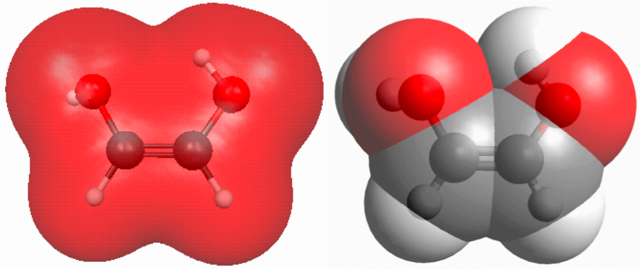
Figure 3.3. (a) RHF/6-31G(d) 0.002 au isodensity surface and (b) van der Waals surface of cis-HO(H)C=C(H)OH (click on the picture for a bigger version).
From Molecular Modeling Basics CRC Press, May 2010.

Looking at the electron density or the van der Waals surfaces one would expect steric strain in cis-HO(H)C=C(H)OH. (See this post on how to make such pictures and this post on how to make an interactive version such as the one shown below.)

However, contrary to CH3(H)C=C(H)CH3, the cis isomer is more stable than the trans isomer. This is of course due to the electrostatic attraction of the O and H atom in the hydrogen bond. Here the electron density tells only part of the story because this attraction involves the nuclei as well. Here an electrostatic potential map is more useful. How to make such plots will be the subject of future posts.

Figure 3.3. The RHF/6-31G(d) electron density of cis-HO(H)C=C(H)OH.
Click on the picture for an interactive version

Friday, December 11, 2009

Common error messages in GAMESS: charge and multiplicity

  *** CHECK YOUR INPUT CHARGE AND MULTIPLICITY ***
THERE ARE 33 ELECTRONS, WITH CHARGE ICHARG= 0
BUT YOU SELECTED MULTIPLICITY MULT= 1
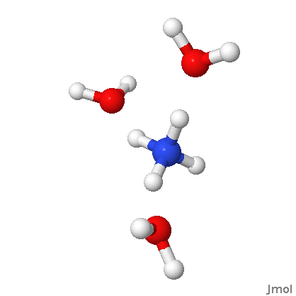
This error message was produced by the following input file. Can you see what's wrong?

$contrl runtyp=optimize $end
$basis gbasis=pm3 $end
$data
Title
C1
N 7.0 -0.39094 1.95659 0.14008
H 1.0 0.38874 1.60529 -0.40413
H 1.0 -0.08386 2.76975 0.70945
H 1.0 -0.72485 1.22934 0.80007
H 1.0 -1.14035 2.30329 -0.48754
O 8.0 -0.64579 0.16732 2.03360
H 1.0 -0.26212 -0.73042 2.10569
H 1.0 -1.00756 0.26750 2.93979
O 8.0 -1.80535 3.31298 -1.59619
H 1.0 -1.39440 3.81065 -2.33214
H 1.0 -2.74148 3.57968 -1.71559
O 8.0 0.26578 4.05264 1.54485
H 1.0 1.03270 4.27032 2.11226
H 1.0 -0.26135 4.87344 1.64760
$end
As GAMESS tells you, it is not possible to have singlet state (i.e. a multiplicity of 1) if you have an odd number of electrons. You need to tell GAMESS whether you want to change the multiplicity (for example, $contrl mult=2 scftyp=rohf $end) or add ($contrl icharg=-1 $end) or remove ($contrl icharg=1 $end).

When looking at the molecule it is pretty clear that you want to remove an electron, since ammonium has a positive charge. So the first line in the input should be changed to
 $contrl runtyp=optimize icharg=1 $end


Click on the picture for an interactive version

Notice that you don't have to specify that the positive charge is on ammonium. The quantum mechanics will take care of that.

Wednesday, December 9, 2009

Electron density and steric strain

Fig3-1-2
Figure 3.2. (a) RHF/6-31G(d) 0.002 au isodensity surface and (b) van der Waals surface of cis-CH3(H)C=C(H)CH3 (click on the picture for a bigger version).
From Molecular Modeling Basics CRC Press, May 2010.

This figure shows how the electron density and van der Waals surfaces can be used to visualize steric strain. See this post on how to make such pictures and this post on how to make an interactive version such as the one shown below.

Figure 3.2. The RHF/6-31G(d) electron density of cis-CH3(H)C=C(H)CH3.
Click on the picture for an interactive version

Tuesday, December 8, 2009

Common error messages in GAMESS: error reading IDUM

 **** ERROR READING VARIABLE IDUM     CHECK COLUMN  1
H 1.0 -0.08386 2.76975 0.70945
....V....1....V....2....V....3....V....4....V....5....V....6....V....7....V....8

This error message was produced by the following input file. Can you see what's wrong?

$contrl runtyp=optimize $end
$basis gbasis=pm3 $end
$data
Title
C1
N 7.0 -0.39094 1.95659 0.14008
H 1.0 0.38874 1.60529 -0.40413
H 1.0 -0.08386 2.76975 0.70945
H 1.0 -0.72485 1.22934 0.80007
H 1.0 -1.14035 2.30329 -0.48754
O 8.0 -0.64579 0.16732 2.03360
H 1.0 -0.26212 -0.73042 2.10569
H 1.0 -1.00756 0.26750 2.93979
O 8.0 -1.80535 3.31298 -1.59619
H 1.0 -1.39440 3.81065 -2.33214
H 1.0 -2.74148 3.57968 -1.71559
O 8.0 0.26578 4.05264 1.54485
H 1.0 1.03270 4.27032 2.11226
H 1.0 -0.26135 4.87344 1.64760
$end
The answer is the missing space in front of the $basis, and the solution is to add a space in front of it, just like for $contrl and $basis.

Why does GAMESS complain about a line in $data when the problem is with $basis? The reason is that it is possible to specify a basis set for each atom in $data, so GAMESS tries to read this information if no $basis group is found.

The error message would clearly benefit from the line: "Did you mean to specify a $basis group?"

Sunday, December 6, 2009

The future of scientific publishing is here today


I recently came across this paper on embedding interactive 3D graphics in pdf files. Unfortunately, I couldn't animate the 3D figures, and I wrote the author (Vlad Vasilyev) who kindly wrote back that:

(1) the publisher (Springer) is a bit behind the times so the interactive figures are found in the supplemental material, but

(2) the ACS is more on the ball, as can be seen in this paper (this is the one I use in the screencast), and

(3) he has made a bunch of tutorials on how to create such diagrams on this page.

This page also contains some pdf files with 3D graphics you can play around with if you don't have access to the papers. Be sure to use Adobe Acrobat Reader 9.

Note that it is also possible to include animations such as vibrational motion (NB: 16 MB file)

Very cool! I haven't tried this myself, but you can be sure I will. Unfortunately, it seems that you need a piece of commercial software (Adobe Acrobat 9 Pro Extended) to do this.

On a related note, check you the interactive figure of interactive figures created by fellow blogger Henry Rzepa (please give the page some time to load).

Sunday, November 29, 2009

Electron density reloaded

Here is an interactive version of a figure I described in a previous post. Click on the picture to load it. Remember it's Jmol so you can rotate it and zoom as you like (Mac users: this works best with Safari).
Figure 3.1. The RHF/6-31G(d) electron density of water.
Click on the picture for an interactive version

The Jmol animation loads this file (h2oprinc.xyz), which looks like this
3
jmolscript: script "http://propka.ki.ku.dk/~jhjensen/h2odensity.spt"
O -0.0000 0.0643 0.0000
H -0.7541 -0.5091 0.0000
H 0.7541 -0.5091 0.0000
and which, in turn, loads a script (h2odensity.spt), which looks like this
isosurface planex plane {0 0 0 0} contour 20 color absolute 0.002 0.05 "http://propka.ki.ku.dk/~jhjensen/h2oprinc.cube.gz"
delay 3
spin y 20
delay 10
spin off
isosurface planey plane {1 0 0 0} contour 20 color absolute 0.002 0.05 "http://propka.ki.ku.dk/~jhjensen/h2oprinc.cube.gz"
spin y 20
delay 10
spin off
isosurface planez plane {0 1 0 0} contour 20 color absolute 0.002 0.05 "http://propka.ki.ku.dk/~jhjensen/h2oprinc.cube.gz"
spin x 40
delay 10
spin off
isosurface threed 0.002 "http://propka.ki.ku.dk/~jhjensen/h2oprinc.cube.gz"
color isosurface red ; color isosurface translucent 0.15
spin y 20
delay 10
spin off
color isosurface red ; color isosurface translucent 0.5
select all; spacefill 100 %babel
spin y 20
delay 10
spin off
The screencast below shows how I made the cube file that contains the electron density information using MacMolPlt. The program I used to convert the MacMolPlt file to a cube was written by Jonathan Gutow and can be download here. In the screencast I mistakenly named the cube file h2odensity.cube.gz, but that's easy to change.

I start by loading the RHF/6-31G(d) optimized geometry I computed for a previous post, and reorienting. The orientation makes it easier to define the plotting plane for the contour plots.

Wednesday, November 25, 2009

Common error messages in GAMESS: No $data

**** ERROR, NO  $DATA   GROUP WAS FOUND
EXECUTION OF GAMESS TERMINATED -ABNORMALLY-
This error message was produced by the following input file. Can you see what's wrong?

$contrl runtyp=optimize $end
$basis gbasis=pm3 $end
$data
Title
C1
N 7.0 -0.39094 1.95659 0.14008
H 1.0 0.38874 1.60529 -0.40413
H 1.0 -0.08386 2.76975 0.70945
H 1.0 -0.72485 1.22934 0.80007
H 1.0 -1.14035 2.30329 -0.48754
O 8.0 -0.64579 0.16732 2.03360
H 1.0 -0.26212 -0.73042 2.10569
H 1.0 -1.00756 0.26750 2.93979
O 8.0 -1.80535 3.31298 -1.59619
H 1.0 -1.39440 3.81065 -2.33214
H 1.0 -2.74148 3.57968 -1.71559
O 8.0 0.26578 4.05264 1.54485
H 1.0 1.03270 4.27032 2.11226
H 1.0 -0.26135 4.87344 1.64760
$end
The answer is the missing space in front of the $data, and the solution is to add a space in front of it, just like for $contrl and $basis.

Saturday, November 21, 2009

Electron density

Fig3-1-1
Figure 3.1.
(a) A contour plot of the density of H2O computed using RHF/6-31G(d). The maximum and minimum contour values are 0.05 and 0.002 aus. (b) The corresponding 0.002 au isodensity surface. (c) The surface corresponding defined by atomic spheres with van der Waals radii.
From Molecular Modeling Basics CRC Press, May 2010.

Here's a screencast about how I made the figure:

When making the contour plot (Figure 3.1.a) I pick 0.05 au as the maximum value (this will be the contour line closest to the nuclei) and 25 contour lines. This means that the spacing between the contour lines and thus the outer contour line will be 0.05/25 = 0.002 au.

Another, more common, representation of the density is a 3D version of one of the contour values: the isodensity surface (Figure 3.1.b). A common choice is 0.002 au, since that corresponds roughly to experimental estimates of molecular size, such as the van der Waals surface (Figure 3.1.c).

Unfortunately, MacMolPlt doesn't have a van der Waals display style, so I have to use Avogadro. This means I have to re-size (by eyeball) this part of the figure to make it the same size as the density plots. See this post about using screen capture to get a file with the graphic.

The interactive version of this figure is the subject of a future post.

The book and color figures

A big part of the motivation for this blog came from writing a book called Molecular Modeling Basics that will be published in May, 2010 by CRC Press. While writing the applications sections it was frustrating to turn the beautifully colored figures into black-and-white versions in order to keep the cost of the book reasonable. But it was also apparent that even colored figures in a book would be a somewhat poor substitute for the interactive versions they are based on. Especially, when turning them around to find just the right orientation for the figure. Wouldn't it be much better to have the reader decide for him/herself?

This is all a long winded way of explaining why there'll be a lot of posts with (color) figures that look like they came out of a book (they'll have figure captions below them). You can click on them for a bigger version. In many of the posts there'll also be a screencast showing how I made them, and an interactive Jmol version. They'll all be labelled "color figures from the book" so they should be easy find.

I always use a screen capture program, rather than saving a graphics file (see the screencast below for an example). I use a free Mac program called Snap and Drag, but I suspect there are plenty of other options for Windows and Linux.

Wednesday, November 11, 2009

A sense of scale


In chapter 1 of volume 1 of the legendary Feynman Lectures on Physics, Feynman starts by imagining zooming in on a drop of water, past amoeba and so forth, until one can see the water molecules. Starting this way is genius. The tiny length scales and the associated invisibility of atoms and molecules is the single largest barrier to developing a chemical intuition - a barrier that molecular animation can help overcome.

I am often thought of bringing Feynman's imaginary magnification to life by animation, so I as very happy when Nathan Baker brought this site to my attention. The above screencast shows it in action, but the real fun is interacting with it yourself. It's a brilliant piece of interactive animation.

The site brought to mind the granddaddy of them all, Powers of 10, which some kind soul put up on youtube.


Monday, November 9, 2009

The trouble with transition metals II: SCF convergence

In a previous post I showed how to build two structural models containing transition metals: a small model of a zinc finger and a ferrocene. This post is about computing the energy using GAMESS.

The first challenge in computing the energy is choosing the correct charge and multiplicity. Most organic molecules are singlets (i.e. all orbitals are doubly occupied) and have an easily identifiable charge. This is often not the case with molecules containing transition metals. Many transition metal atoms have unpaired d electrons and can have several different charges (oxidation states). Also, the charge of the ligands is not always obvious, though they almost always are singlets.

The zinc finger model is relatively easy: zinc is almost always Zn2+ and has 5 doubly occupied d orbitals, so that's a pretty safe bet. The zinc finger model contains two neutral groups (the imidazole rings) and two negatively charged groups (CH3-S-). So the charge of the entire system is zero and the multiplicity is 1.

The ferrocene model is a bit more complicated: iron is commonly found in both the +2 and +3 oxidation state. Before one starts the calculation it is important to find out which one is appropriate for ferrocene. Google says +2 (meaning 6 d electrons) and all doubly occupied orbitals (see the orbitals at the bottom of the page), so a singlet. Furthermore, it is also important to know that each ring has a -1 charge, so the total charge of the complex is 0 and the mutiplicity is 1.

Now, I was all set to talk about SCF convergence problems, i.e. that the zinc finger would converge fine but the ferrocene would give problems. But when I ran a RHF/6-31G(d) energy calculation

$contrl runtyp=energy $end
$basis gbasis=n31 ngauss=6 ndfunc=1 $end
$scf dirscf=.t. $end


both runs converged fine!

"Luckily" when using a smaller basis set (RHF/STO-3G) leads to convergence problems - for both. Here is the relevant part of the SCF output for zinc finger.
                                                                                                                                                                     NONZERO     BLOCKS
ITER EX DEM TOTAL ENERGY E CHANGE DENSITY CHANGE ORB. GRAD INTEGRALS SKIPPED
1 0 0 -3064.6703808712 -3064.6703808712 1.733010527 0.000000000 9751402 457807
2 1 0 -3059.0602240553 5.6101568159 16.724847696 0.794728909 9737106 471195
3 2 0 -3053.0258026844 6.0344213709 16.846293078 0.656307634 9778274 459644
4 3 0 -2935.9005712044 117.1252314800 115.104028436 1.822663152 9792060 446482
5 4 0 -2923.8944526114 12.0061185930 115.740577390 0.620923864 9792989 441267
6 5 0 -2768.2361993103 155.6582533011 115.747362137 5.442595435 9783876 443565
7 6 0 -2921.1390148151 -152.9028155048 115.772970667 0.810505145 9782321 444765
8 7 0 -2775.0326048138 146.1064100013 115.770983819 4.741230605 9783214 444582
9 0 0 -2920.9171138162 -145.8845090024 60.570511833 0.796143103 9783475 444487
10 1 0 -3003.9501726068 -83.0330587906 54.636432025 0.749401761 9790866 444493
11 2 0 -2862.1853212282 141.7648513786 115.095938299 1.824897836 9796139 439522
12 3 0 -2921.4368542174 -59.2515329892 115.495602218 0.722894426 9783664 443903
13 4 0 -2848.2964423996 73.1404118178 115.538938253 2.394847457 9782038 444795
14 5 0 -2905.4155965583 -57.1191541586 115.529755578 0.678236838 9781255 445351
15 0 0 -2859.1068450197 46.3087515386 14.660262004 1.964358011 9783437 444643
16 1 0 -3019.7713654862 -160.6645204665 14.032213984 0.801579670 9794434 443563
17 2 0 -2934.9445251088 84.8268403773 99.891887745 1.748565491 9794346 445610
18 3 0 -2905.6599083961 29.2846167127 100.392269592 1.167341691 9789953 445157
19 4 0 -2864.9366576173 40.7232507788 104.001625891 1.797814244 9781805 446591
20 5 0 -2855.1081148594 9.8285427580 103.862237046 1.447532031 9781260 446026
21 6 0 -2865.3401581051 -10.2320432457 82.200569407 1.143844678 9780463 446052
22 0 0 -2857.7261418857 7.6140162194 78.128990865 1.766124007 9781544 445447
23 1 0 -3036.7926259046 -179.0664840190 5.185277571 0.905312779 9796083 442344
24 2 0 -2977.1610659805 59.6315599241 5.419478057 1.193389134 9796601 444172
25 3 0 -2859.5939849458 117.5670810347 114.799971576 1.724872824 9789000 444821
26 4 0 -2913.7281172708 -54.1341323250 115.553208606 1.094842493 9785096 443663
27 0 0 -2845.9860251842 67.7420920865 16.890315601 1.995942532 9783715 444171
28 1 0 -2989.2091196251 -143.2230944409 16.260193167 1.244487455 9796844 439846
29 2 0 -2911.6240721064 77.5850475187 114.870828357 1.711669748 9798193 439590
30 3 0 -2897.8498052725 13.7742668339 115.443658127 0.704588469 9789911 442464

SCF IS UNCONVERGED, TOO MANY ITERATIONS
TIME TO FORM FOCK OPERATORS= 84.7 SECONDS ( 2.8 SEC/ITER)
FOCK TIME ON FIRST ITERATION= 2.6, LAST ITERATION= 3.0
TIME TO SOLVE SCF EQUATIONS= 0.4 SECONDS ( 0.0 SEC/ITER)

FINAL RHF ENERGY IS 0.0000000000 AFTER 30 ITERATIONS


Clearly, the this SCF is not converging and giving it more iterations is not going to make the problem go away. Instead, different algorithms for SCF convergence are needed and

$scf dirscf=.t. diis=.t. damp=.t. $end

leads to convergence in for both ferrocene and zinc finger.

DIIS stands to Direct Inversion of the Iterative Subspace, which is an extrapolation procedure, while DAMP "damps" any oscillations between in the SCF.

There are a few other tricks to SCF convergence but they are clearly not needed here. If DIIS and DAMP doesn't solve the problem for you, leave a message describing your molecule and I'll see what I can do.

Sunday, November 1, 2009

The trouble with transition metals I: molecule building


This post is long overdue. Quite some time ago (it has been so long I can't find the email anymore) someone asked me to do a post on transition metals.

Modeling of transition metal-containing compounds is notoriously difficult and will require at least two separate posts: one one building the molecules (that's this post) and one on SCF convergence problems.

The screencast shows how to build two molecules: a model of a zinc finger and a substituted ferrocene.

I build the zinc finger model in Avogadro and the only new trick is to pick the UFF force field, because that has parameters for bonds to transition metals.

However, I build ferrocene using Marvin Sketch and import the structure into Avogadro. This is because Avogadro doesn't have multi-center coordination bonds, while Marvin does. The "multi-center" points I add in Marvin Sketch show up as "dummy atoms" in Avogadro. As the name suggests these are not real atoms.

I then use Avogadro to add a functional group to one of the rings and optimize them while leaving the ferrocene part frozen. I could have added the group in Marvin Sketch but Avogadro gives me the opportunity to use autoopt to find the best geometry for the functional group. Note that because I am freezing the transition metal containing part I don't need to assign bonds between the Fe atom and the rings and therefore I can use the MMFF force field, as long as I delete the dummy atoms first.

Sunday, October 25, 2009

Get a reaction: Intrinsic Reaction Coordinate


Lucas requested a post on computing an intrinsic reaction coordinate (IRC). An IRC is a special case of the minimum energy path (MEP) connecting reactant, transition state, and product (more about this at the end of the post).

There are many uses for the IRC, the most basic of which is to verify that the transition state you found actually connects the reactants and products you think it does (this is not always obvious from the normal mode associated with the imaginary frequency). It is also a good way to identify any reaction intermediates you haven't thought about. The IRC is also a way generate an animation of the reaction (see for example ChemTube3D).

An IRC is generated by following the gradient down-hill from the transition state to products and reactants. (It's a bit like a geometry optimization initiated at the transition state, but the algorithm used to follow the gradient is different). Computing a complete IRC thus requires a minimum of two separate runs, and you must find the TS before you can compute an IRC.

The screencast shows how to generate the IRC associated with the 3TSa transition state I found in a previous post. The first input file I generated contain the 3TSa coordinates and the following keywords:

$contrl runtyp=irc $end
$basis gbasis=pm3 $end
$irc saddle=.t. tsengy=.t. forwrd=.t. npoint=100 stride=0.2 opttol=0.0005 $end


saddle=.t. tells GAMESS that the coordinates in $data corresponds to a TS. Because the TS is a stationary point the gradient is zero (or very small), so there is no gradient to follow down-hill. Therefore, the IRC is initiated by displacing the geometry along the normal mode corresponding to the imaginary frequency. Therefore, saddle=.t. GAMESS expects a $HESS group, which contains the frequency information.

Whether the normal mode points towards the reactants or products is completely arbitrary, and the forwrd=.f. keyword is used to change the direction in which the normal mode points. forwrd=.t. is the default and I only include it in the first run for completeness.

tsengy=.t. tells GAMESS to re-compute the energy of the TS (re-compute because you already computed it when you computed the frequencies). If you want to make an energy plot in MacMolPlt as I show in the screen cast, you must set tsengy=.t.

The displaced geometry will have a non-zero gradient, the negative of which points downhill. The geometry is displaced in this direction, the gradient is recomputed, and the procedure is repeated npoint=100 times or until the (root-mean-square) of the gradient is below opttol=0.0005 atomic units, at which point you are at a minimum. (Notice that the default for npoint is 1, and must always be changed).

stride=0.2 tells GAMESS how far along the gradient it should displace at each step (in this case 0.2 atomic units). The default is 0.3, but when I tried this, the IRC calculation in the forward direction failed after 7 steps, because the coordinate deviated too much from the minimum energy path, so I had to decrease it. This means I will have to take more steps to reach the minimum.

As you saw in the screencast, GAMESS takes 100 steps in each direction, which means the IRC does not go all the way to the minimum on each side of the TS. GAMESS does print out restart information to continue the IRC, which I didn't do in this case.

Finally a note on MacMolPlt. As I show in the screencast, MacMolPlt can be used to combine the two IRC runs (forwrd=.t. and forwrd=.f.) by using Files > Add Frames from File... You should first load the file that goes to product and then add the file from the IRC that goes to reactants. Here you should tell MacMolPlt to reverse the order of the structures in the file, so the animation goes from reactions to transition state to product.

This is done by selecting "make these points negative". "Negative" refers to the x-coordinate in the energy plot. The x-coordinate is what separates an IRC from a minimum energy path. An IRC is a plot of the energy of each structure along the minimum energy path vs the root-mean-square change in the mass weighted Cartesian coordinates relative to the TS structure. The TS thus has a x-coordinate of zero, while structures leading to the reactants are defined by negative RMSD values.

If the energy is plotted against something else, such as a bond-length, then it is simply a minimum energy path. Because an IRC uses mass-weighted coordinates, using different isotopes will lead to different IRCs, and one use of IRC is to determine tunneling corrections to the reaction rate.

Saturday, October 24, 2009

Avogadro 1.0 Released

Avogadro - Code Swarm from Marcus Hanwell on Vimeo.

Avogadro 1.0, i.e. the first non-beta version, was released yesterday. The best place to read about this is on Marcus Hanwell's blog (where the movie comes from) and Geoff Hutchison's interview on SourceForge.

The movie (which is best viewed on the vimeo site using full screen) very elegantly shows the evolution of the program (notice the time on the lower right hand side of the screen), from the very beginnings in 2006 when Geoff and Donald Curtis started the project.

For the historians in the audience, Donald has previously worked with me on Ghemical-gms. Ghemical is an open-source model builder based on Babel written by Tommi Hassinen, which Donald made installable on Windows and Mac's to which he added an interface to GAMESS. During the process Donald and Geoff hooked up and the rest, as they say, is history.

Sunday, October 18, 2009

Proteopedia


Proteopedia is just what the name suggests: a wikipedia for proteins. What makes it specific to proteins is the integration of Jmol for animated and interactive figures. It has a long list of pre-made entries ready for use in a lecture and, like a real wiki, you can add content as well.

A lot of the features are explained using a set of very nice screencast. The screencast above is simply a recording of the first 2 minutes of the first video (protopedia does not offer a way to embed the videos) narrated by Eran Hodis.

Wednesday, October 14, 2009

Ribosome Animation

For a while I thought I would be only science blog that would make it through October without mentioning the Nobel Prize. But via Chemical Blogspace I came across this video interview of the 2009 Nobel Prize co-winner in Chemistry Venki Ramakrishnan posted on The Sceptical Chymist (note: spell-check when you name your blog!):
During the interview they show some stunning molecular animations of the ribosome in action, which are credited to Said Sannuga and Ramakrishnan. I wonder ... Sure enough there are several very interesting animations on Ramakrishnan's web site. The screencast above shows a few seconds of one of them. For the rest, go to the site and have a look.

Sunday, October 4, 2009

Building a complicated molecule: meet Marvin


In a previous post I showed how to use PubChem Editor to draw a complicated molecule and import it into Avogadro using the insert SMILES option. Unfortunately, Avogadro does not interpret the chirality information correctly, and chiral structures often have to be fixed.

In the screencast above I show another program, Marvin Sketch, that allows you to draw a structure in 2D and convert it (correctly) to 3D. The coordinates can then be transferred to Avogadro by saving a .mol file.

I also use Marvin to draw 2D structures for the blog. For example

3ts

However, Marvin Sketch is much more than a drawing program. The tools menu contains many powerful cheminformatics tools such as pKa prediction, isomer search, etc.

Marvin Sketch can also be download as a stand-alone program free of charge for academics.

Friday, October 2, 2009

Look who's talking...the ACS

The ACS has released audio recordings synchronized with powerpoint slides of some of the presentations given at the August ACS meeting. A list of the presentations can be found here.

So far, it appears to be free of charge. Let's hope they keep it that way.

Two sets of talks are related to this blog: molecular visualization and animation in chemical education, and I list them here.

I was particularly interested to learn that a GAMESS/VMD interface is well on its way (talk 130-3).

130. Molecular Visualization

130-1 Dr. Michelle M. Kuttel: Visualization of cyclic and multibranched molecules with VMD

Saturday, September 26, 2009

Tunneling and STM


A few weeks ago, I gave a guest lecture (read: "I am at a conference that day, could you do it for me?") in a course entitled Unifying Concepts in Nanoscience. The topic was basic quantum mechanics (chapter 9 and a bit of 10 in Atkin's Physical Chemistry): particle in a box, etc.

These days, the first thing I do when preparing a lecture is to scour Molecular Workbench for useful animations, as I have discussed in a previous post. True to form MW did not disappoint, and I put together the following set of MW slides (note: you need to install MW first before clicking on it).

The screencast above shows how I used four of the slides to illustrate the concept of tunneling and and how it applies to STM.

Once again, I found animated simulations in general, and MW in particular, invaluable in bringing across complex concepts. And once again MW did all the hard work.

2012.09.01 UpdateI made a few more screencasts of parts of my lecture

Sunday, September 13, 2009

The Computational Chemistry Movie


Last week I presented the Computational Chemistry group to the new graduate students, and made the above movie for the occasion. As I mentioned in previous posts (here and here) I think molecular animation is a powerful but overlooked recruiting tool.

Most of the movie is one long Jmol script, but it took some post-editing of the resulting recording to smooth the transitions, i.e. remove the lag time when Jmol is computing the surfaces. The coordinates of the reaction and the large nanostructure is taken from Chemtube3D and this site, respectively. I have described how to extract the coordinates from a site using Jmol in a previous post. The orbitals and vibrational modes were computed using GAMESS and RHF/STO-3G.

The molecular dynamics animation towards the end is done with Molecular Workbench. You can find the simulation here, but you need to install Molecular Workbench to see it.

The equation animation and final credits are done with Powerpoint.

I hope you find the movie entertaining and useful, and feel free to use it (i.e. link to it, embed it, use in a Powerpoint presentation, etc.) if you do. Here is the page in blip.com where you can find the link and the source file in .mov and .flv formats.

Tuesday, September 8, 2009

Hearing voices


While looking for something completely different, I came across this online presentation by Martin Head-Gordon on computational quantum chemistry. The link is here and you click on View Presentation on the right.

The lecture is part of a series on modeling within nanoscience, and the hosting site, nanohub.org, has many other interesting things.

Friday, August 28, 2009

Get a half-life: From transition state to rate constant

hanson08
[source]

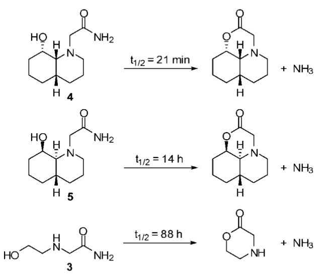
In a previous posts I showed how to find the TS for hydrolysis of 3 at the RHF/3-21G level of theory. In this post I show how to compare the computed results with the experimentally observed half-life (t1/2) of 88 hours.

The half-life is connected to the the rate constant for the reaction (k) by

halflife (1)

The rate constant can be estimated from the activation free energy (ΔG) by transition state theory:

tst (2)

(here the units are those of a unimolecular reaction). The activation free energy is the free energy of the TS relative to the reactant

ΔG = G(3TS) - G(3) = ΔE+ ΔGTRV

Which can be rewritten as the difference in electronic energy and the free energy correction due to translation, rotation, and vibration. I showed how to extract the RHF/3-21G electronic energy (-413.5161 Hartrees) and free energy correction (81.841 kcal/mol) for the 3TSa in a previous post.

In the screencast at the end of the post I show how to obtain the corresponding values (-413.6014 Hartrees and 82.889 kcal/mol) for 3. So,

ΔG(3TSa) = (-413.5161 - (-413.6014))*627.51 + (81.841 - 82.889)
= 52.5 kcal/mol

You can get the corresponding experimental number from the half life (88 hours) and equations (1) and (2): 25.1 kcal/mol and, yep, the RHF/3-21G activation free energy is way off. The corresponding barrier for 3Tsb (51.0 kcal/mol) is only a little better.

There could be many reasons why the activation free energy is so severely overestimated. Two of the most likely suspects are:

1) Level of theory. TS structures, and therefore the underlying wavefunctions, tend to be more complicated than the minima structures. Thus, larger basis sets and electron correlation methods may be needed to obtain accurate activation free energies. This tends to lower the energy of the TS more than the minima, thus lowering the barrier compared to lower levels, but this is not always the case.

2) A different reaction mechanism. What might seem the most straightforward path from reactants to products is not always the one with the lowest barrier. For example, in the case of amide hydrolysis a stepwise mechanism is also possible in which the hydroxyl hydrogen is transferred to the carbonyl O atom to create a (chiral) intermediate.

amideint

TSs corresponding to such a mechanism must also be found to see if they lead to lower activation free energies. If you followed the last few posts of finding TSs you now have all the skills needed to do that.


Here is the screencast that shows how to find the energies for 3:


I paste in the following set of keywords

$contrl runtyp=optimize $end
$system mwords=125 $end
$statpt opttol=0.0005 nstep=50 hssend=.t. $end
$force nvib=2 $end
$contrl nzvar=1 $end
$zmat dlc=.t. auto=.t. $end


In the RHF/3-21G optimization + frequency run I forgot to add

$scf dirscf=.t. $end

which would have speeded up the calculation, as I described in a previous post.

Thursday, August 20, 2009

GAMESS, memory and parallel


The screencast above is a repeat from the last post, where I computed the frequencies of a molecule at the RHF/3-21G level of theory (second screencast) and discovered that the amount of memory that GAMESS requests (1,000,000 words) was not enough. While GAMESS tells me how much it needs in the output file, it does so after a lot of computation, which is wasted because I have to start over.

In this post I discuss the basics of GAMESS memory requirements. The simplest case is when you are not running in parallel, i.e. the number of processors in GAMESSQ is set to 1, so I discuss this case first.

1. Memory is specified in $system, and the default is 1 mega-word (i.e. 1,000,000 words):

$system mwords=1 $end

mword can only be integers (1, 2, 3, ..). (In the screencast above I used the older "memory" keyword but mwords is much more convenient.)

2. A word is 8 bytes, so the default memory request (1 mega-word) is a very modest 8 MB of RAM.

3. This is the maximum amount of memory GAMESS is allowed to use. Depending on the type of calculation GAMESS might use less. The option is there to avoid filling up the memory on the computer entirely, which will crash or freeze the computer.

4. Here is the simplest way to deal with memory: My current laptop computer has 2 GB of RAM, and I use it for other things while GAMESS is running, so I am willing to give GAMESS a maximum of roughly 1 GB of RAM. This translates to

1 GB ≈ 1,000 MB ≈ 125 mwords

5. Adding

$system mwords=125 $end
to all input files will allow me to run most GAMESS jobs that I would want to run on a laptop without ever getting a "not enough memory" error (of course if you have less memory you need to adjust mwords accordingly).

That's basically it. What follows is some more details that most casual users of GAMESS won't have to worry about.

6. Most common GAMESS runs will never get close to using 1 GB of RAM, meaning the memory is free to be used by other programs. The most common types of runs that potentially could use that much memory are frequency calculations using RHF and any kind of MP2 calculation. Slightly less common ones are TDDFT and NMR calculations. In GAMESS, DFT frequency calculations are done numerically, and do not require a lot of memory.

7. If you are in doubt whether you have reqeusted enough memory to perform a calculation it is possible to use GAMESS to check using

$contrl exetyp=check $end


This keyword will simulate an actual GAMESS run by skipping the most time consuming steps so it is very fast.

I show two examples (an RHF/3-21G frequency and MP2/6-31G(d) single calculations on 3TSa) in this screencast.


Parallel runs

8. Many desktop computers (and almost all larger computers) have more than one CPU (also known as cores). For example, my current laptop has one processor with 2 cores. Thus, I could make my GAMESS calculations go faster by specifying 2 processors when submitting with GAMESSQ (processor = core in GAMESS-speak). This means that two separate but related GAMESS calculations are running simultaneously, and this affects the memory request:

9. Most types of runs use replicated memory. This means that if mwords=1 but I ask for 2 processors, GAMESS will use a maximum of 2 mega-words. Thus, if I routinely use 2 processors when running on my laptop and want to impose a limit of 1 GB RAM, I should use

$system mwords=63 $end

instead of 125.

10. The most common exception to this is MP2 calculations, where GAMESS uses both replicated (mwords) and distributed memory (memddi). Distributed memory is memory shared by the cores. If I specify memddi=100 and ask for 2 processors then 100 mega-words of RAM is distributed among the 2 processors (the simplest case is that each core gets 50 mega-words, but GAMESS figures that out for you).

So running on 2 processors with

$system mwords=15 memddi=100 $end
requests a total of (15 + 15 + 100 =) 130 mwords. You can use exetyp=check to figure out the optimum values of memory and memddi, as I show in this screencast.


The screencast shows how you can use 1 processor and

$contrl exetyp=check $end
$system memddi=100 parall=.t. $end


to check the memddi requirements. You need to make memddi large for this to work, but GAMESS will not use this memory during the check-run. Note that parall only "does something" for check runs: true parallel runs are specified by choosing more than 1 processors when you submit GAMESS.

You can get a complete list of runs that require memddi in Chapter 2 of the GAMESS documentation under the entry for $system. Also, Chapter 5 has a more in-depth description of how memory is handled.

Friday, August 14, 2009

Finding a transition state: amide hydrolysis 2


In a previous post I found two TSs, called 3TSa and 3TSb, at the PM3 level of theory.

In this post I show how the PM3 structure and frequency information can be used as a starting point for finding 3TSa at the RHF/3-21G level of theory.

I use RHF/3-21G as an example of an expensive ab initio method where we want to keep the number of frequency calculation to a minimum, since it takes a long time to compute.

So I extract the PM3 optimized geometry from the output file of the TS search, and add to this the corresponding frequency information in the form of the $HESS group from the .dat file.

The keywords I paste in look like this (many of these keywords have been described in a previous post):

$contrl runtyp=sadpoint $end
$scf dirscf=.t. $end
$statpt opttol=0.0005 nstep=50 $end
$statpt hess=read $end
$contrl nzvar=1 $end
$zmat dlc=.t. auto=.t. $end


Note the $basis group is missing, but that I specify it using Avogadro. It's important to pick the basis set before pasting the remaining keywords in because Avogadro deletes some of the lines in the file when you select something in the menu.

Based on the PM3 guess, GAMESS finds the RHF/3-21G TS in 29 steps.

Actually, I can't be 100% sure the structure is a TS because I haven't verified that the structure has an imaginary frequency. Unlike with PM3 I don't automatically compute the frequencies at the end of the TS search (using hssend=.t.).

The reason is that it is a good idea to verify that the structure looks like a TS before committing CPU time to an expensive frequency calculations. As I showed in a previous post it can happen that TS searches end up find the reactants and products.

Luckily the TS structure has one, and only one imaginary frequency as you can see in this screencast


As you saw the default amount of memory that GAMESS requests (1,000,000 words) is insufficient for the RHF/3-21G frequency calculation, but it tells you how much it needs (~1,100,000 words). A "word" is 8 bytes, so we are talking about 10 MB here. I will discuss this issue in more details in a future post.

Finally, in principle it is possible to adjust the memory keyword in Avogadro (in the Advanced setup), but that option is currently not working.

Now we need to repeat this procedure for 3TSb. The procedure are exactly the same, so I haven't made a screencast. The TS search takes 36 steps.

Monday, August 10, 2009

GAMESSQ for everyone

When I made the post about GAMESSQ, I had no idea it was only being distributed for the Mac (together with the Mac binary) - I usually don't make posts on software that is not cross-platform.

However, now Brett Bode has made a general release of GAMESSQ. Here you can find a Windows executable and the source code, the later being the only current option for Linux users.

It is not inconceivable that one or two Linux binaries will be available soon. What flavor if Linux would be most useful to MolModBasic readers?

Sunday, August 9, 2009

Finding a transition state: amide hydrolysis I

hanson08
In a previous post I showed how to find a TS for an Sn2 reaction involving a small molecule (it's a good idea to look at this post now if you haven't seen it before, and check out this post as well).

In this and future posts I discuss the steps involved in finding a TS for a reaction involving complicated molecules shown in the figure above (I have shown how to build some of the reactants in a previous post).

Say you want to find the TS for the hydrolysis of 4 and 5 at a relatively high level of theory. My advice is to start by finding the TS at a low level of theory (PM3) for a smaller representative reaction (hydrolysis of 3). This is the subject of today's post.

The basic procedure is the same as in the previous post:

1. I build a TS-like structure by constraining a key distance during an energy minimization.
2. I check whether the optimized geometry has an imaginary frequency that looks like the reaction coordinate
3. If it does, I use it as a starting point for the TS search.

In the previous example, one bond broke as the other one formed, so I simply forced one bond (the C-F bond) to form by constraining it to 2.0 Å and the optimization took care of the rest.

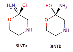
In the hydrolysis of 3, two bonds have to break (the C-N and O-H bonds) as two other bonds form (the C-O and N-H bonds), so what to constrain? In general I have found it a good idea to try to construct an intermediate structure, such as "3TSa" shown below.
3ts
Here the O-H bond is already broken and the C-O and N-H bonds are already formed. The question is now reduced to whether I should try to break the C-O or the C-N bond. I opted for the C-O bond which I start breaking by constraining it to 2.0 Å. The reason for choosing the C-O bond is that I assumed that the (potential) energy of 3 is lower than the products (because of ring strain) so the TS should be more product-like according to Hammond's postulate (you can of course check this computationally).

Why do I pick 2.0 Å? Well, you have to start somewhere and this is a nice round number (for bonds involving 3rd row atoms I would use 2.5 Å). As you see in the screencast below, 2.0 Å doesn't work but the TS search tells me how to change it, i.e. increase it to make it more reactant like as the TS search goes to products.


As you saw in the screencast I have pre-typed some text with keywords that I use again and again, and simply paste the text in the input file and alter it when necessary. For the constrained optimization the text looks like this:

  $contrl runtyp=optimize $end
  $basis gbasis=pm3 $end
  $statpt opttol=0.0005 nstep=50 hssend=.t. $end
  $force nvib=2 $end
  $contrl nzvar=1 $end
  $zmat dlc=.t. auto=.t. ifzmat(1)=1,x,x fvalue(1)=2.00 $end


and for the TS search the text looks like this.

  $contrl runtyp=sadpoint $end
  $basis gbasis=pm3 $end
  $statpt opttol=0.0005 nstep=50 $end
  $statpt hess=calc ihrep=5 hssend=.t. $end
  $force nvib=2 $end
  $contrl nzvar=1 $end
  $zmat dlc=.t. auto=.t. $end


You might also notice that I am being a "CPU slob" in the sense that I redo some computations I've already done. For example, I compute the frequencies for the optimized constrained geometry twice: at the end of the optimization and at the beginning of the TS search. That is because I am using PM3, which is such an efficient method that the computer can re-compute the freqeuncies in less time than it takes me to transfer the $HESS group to the TS search input file (as shown in a previous screencast)! Similarly, when I find that 50 steps is insufficient and just restart with nstep=100 steps, which recomputes the first 50 steps. Good thing sloth is not a deadly sin.

Another advantage of constructing a hypothetical intermediate in this case is that you realize (hopefully) that the TS contains a chiral center, even though the reactants and products are achiral. So you have to look for two TSs, to see which one is lowest in energy.

The next screencast shows how I find 3TSb, which is made easier by the fact that I have a good idea of what the constraint value should be (2.32 Å) from the 3TSa geometry I found previously.

Sunday, August 2, 2009

Finding a transition state: an Sn2 reaction


Here is a screencast I made about finding a transition state for the reaction

F- + CH3Cl -> Cl- + CH3F

The general approach is as follows

1. Build the structure (F- + CH3Cl)
2. Optimize the geometry while constraining a key distance (between the F and C atom) to a certain value (2.0 Å)
3. Compute the frequencies for the optimized geometry to check for an imaginary frequency
4. If there is an imaginary frequency, use this geometry and frequency information as a starting point for the TS search

The distance constraint is imposed using

$zmat ifzmat(1)=1,1,6 fvalue(1)=2.0 $end

which is used in conjunction with the delocalized internal coordinates I discussed previously. 1,1,6 defines the distance (denoted with the first "1") between atoms 1 and 6. Note that this distance does not have be 2.0 Å in the guess geometry (though the closer it is to 2.0 Å the faster the optimization will converge).

I also show how the frequency information contained in the $HESS group, found at the end of the .dat file that GAMESS produces along with the output file, can be transferred to the input file for the TS search, where hess=read is used in $statpt. Any text editor can be used for this. Note that the hssend=.t. keyword has to be used to cause the frequencies to be computed at the end of the optimization. I have showed the use of this keyword in a screencast in a previous post.

The complete $statpt groups looks like this

$statpt opttol=0.0005 nstep=50 hess=read ihrep=5 hssend=.t. $end

ihrep=5 causes the frequencies to be recomputed at every 5th step. This really helps convergence but is computationally expensive.

Note that there are no constraints imposed when searching for the TS.

The key question is of course why I chose the C-F distance and 2.0 Å for the constraint value. This is simply the first thing that popped into my head and it happened to work. If it hadn't, I would have tried some other values and, if none worked, I would have tried to the C-Cl distance. Future posts will show examples of trying difference distances.

Because you may have to try different constraints before succeeding, it is a good idea to find the TS at a cheap level of theory, such as PM3. The C-F distance in the PM3 TS structure (2.10 Å) should provide a good guess for TS searches at higher levels of theory.

I tried it for this reaction using RHF/3-21G, but with no luck. That is because I forgot the very first step in searching for a TS: make sure there is one! In the screencast below I show how a RHF/3-21G geometry optimization (with no constraints) starting from F- + CH3Cl leads to Cl- + CH3F, meaning that the former structure is not a minimum on the gas phase RHF/3-21G potential energy surface. So there is not much point in looking for the corresponding TS.

Saturday, July 25, 2009

A typical set of GAMESS calculations


In this post I show the sequence of GAMESS calculations necessary to compute the free energy of the water dimer molecule at the B3LYP/6-31G(d)//PM3 level of theory. This notation means that the geometry and the free energy contribution is obtained with PM3, while the electronic energy is computed using B3LYP/6-31G(d) and the PM3 geometry. (By default the free energy is computed at 298.15 K and 1 atmosphere pressure.)

The steps are as follows:

1. Build the molecule

2. Optimize the geometry using PM3

3. Compute the frequencies for the optimized geometry to
a. verify that you found a minimum
b. compute the sum of the translational, rotational, and vibrational free energies at the PM3 level.

4. Compute the B3LYP/6-31G(d) energy for the PM3 optimized geometry

Some of the keywords I used have been described in a previous post, and I actually copy the keywords from this post to save typing.

The electronic energy for the water dimer is -152.7533 atomic units (au) while the sum of the translational, rotational, and vibrational free energies is 13.820 kcal/mol. If you repeat these calculations for the water molecule you get -76.3715 au and 2.271 kcal/mol (1 au = 627.51 kcal/mol).

So, the change in electronic energy on going from two water molecules to the water dimer is

ΔE = (-152.7533 - 2(-76.3715))*627.51 = -6.4 kcal/mol

The corresponding free energy change is

ΔG(298K) = -6.4 + 13.820 - 2(2.271) = -6.4 + 9.3 = 2.9 kcal/mol

Here I make the usual assumption that the electronic free energy is the electronic ground state energy.

Notice that the free energy change is positive meaning the water dimer is not predicted to form at this temperature and pressure (1 bar) under equilibrium conditions (the relative probability of observing the water dimer can be computed with this equation). This is because of the entropy of loss on going from 2 particles to 1.

Friday, July 24, 2009

Some GAMESS input basics

Update 2 August 2009: I have changed the discussion regarding the SG1 keyword. New text is in italics.

I have planned some posts in which some details of the GAMESS input will become important, so this post is about the basic anatomy of a GAMESS input file, and some non-default settings that I use all the time.

Here is an input file for a single point energy calculation at the B3LYP/6-31G(d) level of theory for the H2 molecule:

$contrl runtyp=energy dfttyp=b3lyp $end
$basis gbasis=n31 ngauss=6 ndfunc=1 $end
$data
Title line: you can write anything here
c1
H 1.0 0.0 0.0 0.0
H 1.0 0.753 0.0 0.0
$end


• The order of the groups doesn’t matter, so you can put the $basis group below the $data group.

• You can have several groups of the same kind (e.g. two $contrl groups). If you have the same keyword in both groups, it is the value in the last group that counts. For example,

$contrl runtyp=energy dfttyp=b3lyp $end
$contrl runtyp=optimize $end

is perfectly legal, and will result in an geometry optimization.

• The order of the keywords within a group doesn’t matter.

$contrl runtyp=energy dfttyp=b3lyp $end

is the same as

$contrl dfttyp=b3lyp runtyp=energy $end

• Note that there is a space in front of any line starting with a $ sign. This is important and if you leave it out GAMESS will not read that line. Note you can use this to “uncomment” a line by adding, for example, a ! For example, this

$contrl runtyp=energy dfttyp=b3lyp $end
!$contrl runtyp=optimize $end

will result in a single point energy calculation

• You can use capital letters if you want.

• For parameters that can be true for false, you can use either “.true.” or “.t.” and “.false.” or “.f.” (there's an example below).

• A line can only be 80 characters long. Anything after that is ignored. It is perfectly legal to split a line, for example:

$contrl runtyp=energy
dfttyp=b3lyp $end


Some useful options

Almost all of the parameters have default (but there is no default basis set and no defaults in $data). For example, the default runtyp is energy, so

$contrl dfttyp=b3lyp $end

will result in a single point energy evaluation. If $contrl is missing entirely, GAMESS will compute a single point energy at the RHF level.

There is a few defaults that I almost always change

Single point energy calculations (not AM1 or PM3)

$scf dirscf=.t. $end

This tells GAMESS to recompute the integrals at each SCF step rather than reading them from hard disk. Most computers can recompute a number faster than they can find it on the hard disk.

DFT single point energy calculations

$dft sg1=.t. $end

Computing the DFT energy requires a numerical integration over a grid. The default grid is very fine (has a lot of points). Standard Grid 1 (sg1) is adequate for most purposes and much faster. Note that this leads to inaccurate gradients and should not be used for geometry optimizations.

DFT, AM1, and PM3 frequency calculations

$force nvib=2 $end

DFT and semiempirical Hessians (second energy derivatives) are computed numerically, by displacing each atom in the x, y, and z direction and computing the first derivative. This is usually not accurate enough. nvib=2 leads to a displacement in both the positive and negative x, y, and z direction resulting in more accurate frequencies.

Geometry optimizations

$statpt opttol=0.0005 nstep=50 $end
$contrl nzvar=1 $end
$zmat dlc=.t. auto=.t. $end


I think the default criterion for geometry convergence (0.0001) is too strict, and the default number of steps (2o) is too small. So I usually use 0.0005 and 50, respectively. Optimizing in internal coordinates instead of Cartesian coordinates (default) usually speeds up convergence, because the former are "more quadratic". nzvar=1 tells GAMESS to use internal coordinates and dlc and auto tells GAMESS to automatically generate delocalized internal coordinates.

Unfortunately, the DLC implementation in GAMESS only looks for covalent bonds, not H-bonds and such. So you have to specify these if you have specify non-covalently bonded molecules in the input file. For example, in the case of water dimer (see figure for numbering), you do it like this

$zmat nonvdw(1)=1,4 $end

Note that you don't have to specify the H-bond in HO-CH2-CH2-OH, since the OH groups are connected by covalent bonds.

So, an input file for a geometry optimization of the water dimer would look like what I show below. That might seem a lot to type, but the trick is of course to type is once, store it somewhere handy, and copy it into new files.

$contrl runtyp=optimize dfttyp=b3lyp $end
$basis gbasis=n31 ngauss=6 ndfunc=1 $end
$scf dirscf =.t. $end
$statpt opttol=0.0005 nstep=50 $end
$contrl nzvar=1 $end
$zmat dlc=.t. auto=.t. nonvdw(1)=1,4 $end
$DATA
Title
C1
O 8.0 -4.42170 -0.11056 -2.11879
H 1.0 -3.53334 -0.03874 -1.70405
H 1.0 -4.75257 0.79398 -2.01675
O 8.0 -2.06207 0.35222 -0.78539
H 1.0 -1.13417 0.41136 -1.06880
H 1.0 -1.98676 0.07447 0.14406
$END